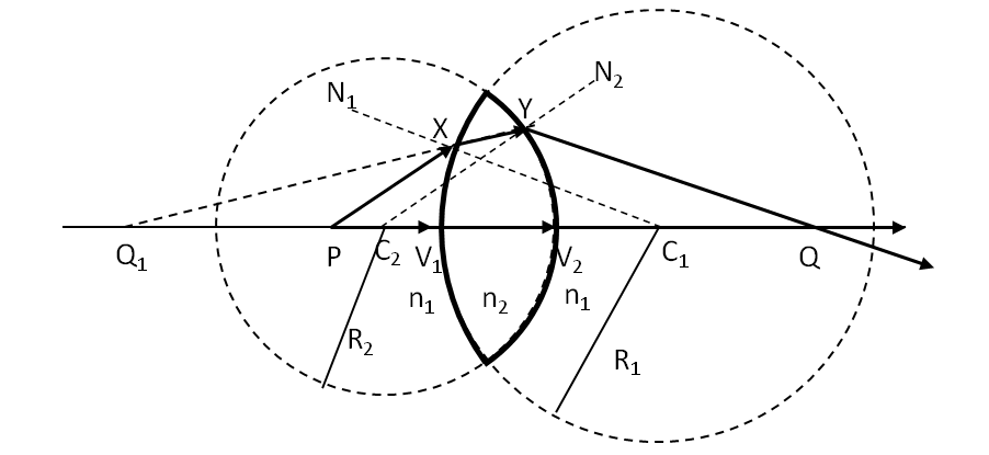
To study lens analytically, we can make use of our results from refraction at one spherical interface. For concreteness, we will look at a biconvex lens with refraction of light at the two interfaces of a lens as shown in Figure 2.55.
For illustrative purposes, we choose a point object P on the symmetry axis of a bi-convex lens. Let the refractive index of the surrounding media be \(n_1\) and that of the lens be \(n_2\text{.}\) Let the radii of curvatures of the two sides be \(R_1\) and \(R_2\) as shown in the figure. We wish to find a relation between the object distance, the image distance and the parameters of the lens. This relation is called lens-maker’s equation.
Figure2.55.Image formation in a lens. Here d is the thickness of lens. We shall take \(d \ge 0\) limit to obtain formula for thin lens. In thin-lens approximation \(d=0\text{.}\)
Locating the Final Image Graphically: Locating the image graphically as a result of refraction through a lens is straightforward. As usual we draw two rays of light \(\text{PV}_1\text{V}_2\text{Q}_1\) and \(\text{PXYQ}\) tracing their paths through the lens making sure to take into account the refractions at the interfaces according to the Snell’s law. We find that the rays intersect at point \(\text{Q}\) for the case shown in Figure 2.55. The crossing of real rays at point Q generate a real image there.
Details of Images at Two Refractions:
Image \(\text{Q}_1\) by Refraction at First Interface: We now examine the path \(\text{PXYQ}\) in Figure 2.55 more closely. The incident ray PX bends towards normal and goes in the direction XY inside the glass, but it is diverging away from the inside path \(\text{V}_1\text{V}_2\) on the axis, therefore we need to extend XY backward to axis meeting it at \(\text{Q}_1\) which is a virtual image of P created by the front surface of the lens. The image \(\text{Q}_1\) is image due to refraction at the front surface.
Image \(\text{Q}_1\) by Refraction at First Interface: When the rays XY and \(\text{V}_1\text{V}_2\) reach the second surface of the lens, they refract at that surface. This situation is similar to the rays originating in the medium \(n_2\) which extends to infinity on the left of the second interface and refracting into the medium \(n_1\text{.}\) [By the way, the medium to the right does not have to have the refractive index \(n_1\text{.}\) We are using the same refractive index on the two sides of the lens to keep our formulas simpler.] The rays XY and \(\text{V}_1\text{V}_2\) can be considered to come from the same point \(\text{Q}_1\) in medium of refractive index \(n_2\text{.}\) Actually, all rays starting from P and having refracted at the front surface would appear to be coming from \(\text{Q}_1\) as far as the second interface of the lens is concerned.
Image \(\text{Q}\) by Refraction at Second Interface: The ray XY refracts in the direction YQ and meets the ray \(\text{Q}_1\text{V}_1\text{V}_2\text{Q}\) on the axis. To find the location of the image point \(\text{Q}\) graphically we need to draw the figure as precisely. However, there is also an algebraic method of analysis that gives algebraic relations which is often easier to use that to draw rays. We still draw rays to get an overall picture but do the calculations using the algebraic equations to obtain quantitative values.
Locating the Final Image Analytically: Various distances in Figure 2.55 will be denoted by the following symbols.
The algebraic method relies on the refraction formulas for the spherical surfaces we have obtained in the last section. First we locate the image \(\text{Q}_1\) due to the refraction at the first interface, and then use \(\text{Q}_1\) as an object for the second interface to find the final image at Q.
We have the following additional relation. The object distance for the second interface is from \(\text{V}_2\) to \(\text{Q}_1\text{,}\) and since \(q_1\) is negative, i.e., \(q_1 \lt 0\text{,}\) the distance \(p_2\) will depend on \(q_1\) and the width \(d\) of the lens.
Note that \(q_1\) is a negative number here, therefore \(-q_1\) is positive. Put \(p_2\) from Eq. (2.29)into Eq. (2.28) and add Eq. (2.27) and Eq. (2.28) to obtain the following.
In the \(d \rightarrow 0\) limit, which is also called the thin lens approximation, the last term goes to zero, and \(\text{V}_1\) and \(\text{V}_2\) become one point. All distances are then measured from the center of the lens rather than either vertex. We can drop the subscripts on \(p\) and \(q\) since the distances are measured from the center.
This equation is called the lens maker formula. This formula has the same form as \(\frac{1}{p} + \frac{1}{q} = \frac{1}{f}\) if we identify the right side as \(1/f\text{,}\) where \(f\) is the focal length of the lens.
Since \(n_l \gt 1\text{,}\) the sign of the focal length depends on the sign of the result of calculation of quantities in the parenthesis. Thus, for bi-convex lens (\(R_1 \gt 0\text{,}\)\(R_2 \lt 0\)), you will always get postive \(f\) and for bi-concave lens (\(R_1 \lt 0\text{,}\)\(R_2 \gt 0\)), you will always get negative \(f\text{.}\) For some other mixed curvatures the sign of \(f\) will depend on the actual values of curvatures. If \(f\) is positive we call the lens converging lens and if negative diverging lens.
In most applications, we are given focal length with type of lens, whether converging or diverging, and we don’t need to worry about the dimensions of the lens. This shows that in the thin-lens approximation, with all distances measured from the center of the lens, following formula applies.
Object focal point \(\text{F}_1\) and image focal point \(\text{F}_2\) are symmetrically placed for thin lenses, i.e., they are at an equal distance from the lens as illustrated in Figure 2.56.
Figure2.56.First and second foci of lenses.
Remark2.57.Thick Lenses:.
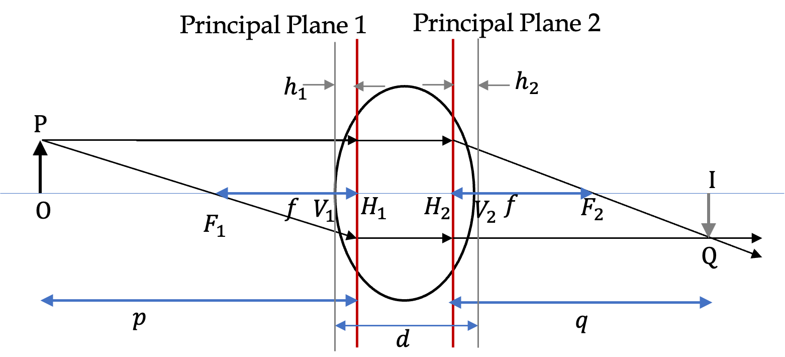
Notice that without the thin lens approximation, the right side of the equation has terms containing the position of the intermediate image from the front vertex that doesn’t soleley depend upon the dimensions and refractive index of the lens and the medium. In a later courses when we study thick lenses, you will find that a more complex rules for measuring distancs as shown in Figure 2.58 leads to the right side just truly be just a property of the lens and the medium alone.
Figure2.58.Rays through a thick lens. Distances measured from the principal planes give rise to simpler formulas.
For the sake of simplicity, let the lens be surrounded by air/vacuum so that \(n_1=1\) and let us use symbol \(n_l\) for the refractive index of the lens. With focal length measured from the principal planes, the formula for the power of the lens is
\(p\) positive if left of the lens otherwise negative.
\(q\) positive if image to the right of the lens otherwise negative.
\(f\) positive for convex lens and negative for concave lens.
By using a finite size object on the axis you can prove that the magnification of image defined as the ratio of the image height to the object height is equal to the negative of the image distance to object distance \(-q/p\text{.}\)
Transverse Magnification \(M_T\) The size and orientation of the image with respect to the image is given by the magnification \(m\) defined as the ratio of image height \((h_i)\) to the object height \((h_o)\text{.}\)
If magnification is negative then image is inverted with respect to the object. By using the geometry of the rays you can show that the ratio of the heights are related to the ratio of the image distance and the object distances.
For the sake of brevity, we will often write \(m\) for \(M_T\text{.}\)
\begin{equation*}
M_T \equiv m.
\end{equation*}
Example2.59.Location and Magnification of Image from a Convex Lens.
Find the location, orientation and magnification factor of the image in each of the following positions of an object of height 3 cm in front of a convex lens of focal length 10 cm. (a) \(p = 50\text{ cm}\text{,}\) (b) \(p = 5\text{ cm}\text{,}\) (c) \(p = 20\text{ cm}\text{,}\) (d) \(p=10\text{ cm}\text{.}\)
Inverting this, we get \(q = 12.5\text{ cm}\text{.}\) Since \(q\) is positive, the image will form on the right of the lens. This will give us a real image. The magnification of the image can be obtained from \(p\) and \(q\text{.}\)
The negative magnification means that the image would be inverted. Furthemore, since \(|m_T|\lt 1\text{,}\) the image would be shorter than the object. The size of the image is given by
Therefore, \(q = -10\text{ cm}\text{,}\) which is negative, meaning the image is on the left side of the lens, the same side as the object. The magnification of this image
The positive magnification means that the image would be upright, the same orientation as the object. Since \(|m_T|>1\text{,}\) the image would be larger than the object, i.e. the image will be magnified. The size of the image is given by
The negative magnification means that the image would be inverted. Since \(|m_T|=1\text{,}\) the image would be of the same size as the object. The size of the image would be given by
Here, we are placing the object at the first focal point of the lens. We expect the outgoing rays from the lens will be parallel in all directions. This will mean the image will be very far away, i.e., at infinity. Let’s see how the algebra works out.
Therefore, \(q=\infty\text{.}\) From \(m_T=-q/p\text{,}\) we get \(m_T=-\infty\text{.}\) That means if you are a little bit inside a focal length, image will be virtual, have same vertical orientation, and will be magnified considerably. however, if you were a little but further than the focal point, the image will be real, far away and inverted in orientation. So, the negative sign in \(m_T=-\infty\) is a little bit deceptive since if you are right at the focal point, the image will be at infinty, which means there will be no image at all.
Example2.60.Location and Magnification of Image from a Concave Lens.
Find the location, orientation and magnification factor of the image in each of the following positions of an object of height 3 cm in front of a concave lens of focal length 10 cm. (a) \(p = 50\text{ cm}\text{,}\) (b) \(p = 5\text{ cm}\text{,}\) (c) \(p = 20\text{ cm}\text{,}\) (d) \(p = 10\text{ cm}\text{.}\)
Answer.
(a) \(q = -8.33\text{ cm}\text{,}\)\(m_T=+\frac{1}{6}\text{,}\) same vertical orientation, \(0.5\ \text{cm}\text{.}\) (b) \(q = -3.33\text{ cm}\text{,}\)\(m_T=+\frac{2}{3}\text{,}\) same vertical orientation, \(2\ \text{cm}\text{.}\) (c) \(q = -6.67\text{ cm}\text{,}\)\(m_T=+\frac{1}{3}\text{,}\) same vertical orientation, \(1\ \text{cm}\text{.}\) (d) \(q = -5\text{ cm}\text{,}\)\(m_T=+\frac{1}{2}\text{,}\) same vertical orientation, \(1.5\ \text{cm}\text{.}\)
Solution1.(a)
(a) In this part we have \(p = 50\text{ cm}\text{,}\) and \(f = -10\text{ cm}\text{,}\) and we are looking for \(q\text{.}\) Therefore,
Inverting this, we get \(q = -8.33\text{ cm}\text{.}\) Since \(q\) is negative, the image will form on the same side of the lens as the object. This will give us a virtual image. The magnification of the image can be obtained from \(p\) and \(q\text{.}\)
The positive magnification means that the image would have same vertical orientation as the object. Furthemore, since \(|m_T|\lt 1\text{,}\) the image would be shorter than the object. The size of the image is given by
Therefore, \(q = -3.33\text{ cm}\text{,}\) which is negative, meaning the image is on the left side of the lens, the same side as the object. The magnification of this image
The positive magnification means that the image would be upright, the same orientation as the object. Since \(|m_T| \lt 1\text{,}\) the image would be shorter than the object, i.e. the image will be diminished in size. The size of the image is given by
Therefore, \(q = -6.67\text{ cm}\text{.}\) The negative image distance means the image is on the left side of the lens, i.e. on the same side as the object.
Therefore, \(q = -5\text{ cm}\text{.}\) The negative image distance means the image is on the left side of the lens, i.e. on the same side as the object.
Note that unlike the case with the convex lens, placing the object at the first focal point did not result in image at infinity!
Example2.61.Carving a Bi-Concave Lens for a Given Focal Length.
Suppose you have been asked to make a bi-concave lens of focal length \(-20\text{ cm}\) in air.
(a) Find the radius of curvature of a symmetrically ground biconcave lens from a glass of refractive index \(1.55\) assuming you can ignore the thickness of the lens.
(b) If the lens is used underwater, what will be refractive index of the lens then?
In a biconcave lens, the radii will have the following signs: \(R_1 \lt 0\text{,}\) and \(R_2 \gt 0\text{.}\) You can convince yourself by drawing a picture and applying the sgn convention. Now, here \(|R_1|=|R_2|\text{.}\) Lets use a common symbol \(x \gt 0\) for this absolute value in Eq. (2.33). Therefore,