AC Source

Section 44.1 AC Source

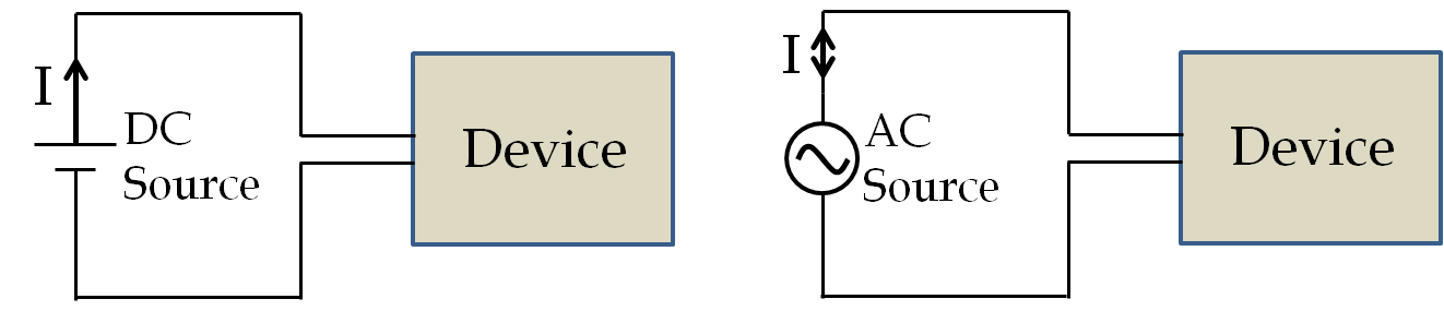
Alternating current (AC) circuits form the backbone of distribution of electricity to households and industry. The behavior and analysis of AC circuits are very different than Direect Current (DC) circuits, so you would have to learn anew how to calculate currents and voltages in an AC circuit. To start with, a current in DC circuit always points in the same direction, but in an AC circuit, the direction of current changes with time as illustrated in Figure 44.1.1.

Figure 44.1.1. In a direct current (DC) the direction of current remains fixed in time. In an alternating circuits (AC) the direction of the current changes with time.

In this chapter we will study AC circuits where the current in a circuit is driven by an oscillating electromotive force, which we will refer to as voltage. We are going to use symbol \(V\) instead of symbol \(\mathcal{E}\) for EMF and voltage.

\begin{equation*} V(t) = V_0 \cos(2\pi f t + \phi), \end{equation*}

where \(V_0\) is the amplitude of the oscillating voltage, \(f\) the frequency of oscillations, and \(\phi\) the phase constant. Amplitude \(V_0\) is also called peak voltage of the source. The argument of cosine, here \((2\pi f t + \phi)\) is called the phase of the source. Sometimes the phase constant \(\phi\) itself is called the phase.

If there is only one source we pick the zero of time such that \(\phi\) can be set to zero. But, if you have two or more sources, such as in common three-phase line discussed below, their phase constants may be different even when the sources may fluctuate with the same frequency. In that case, the phase constant gives us important information about the relative timings of peaks and troughs of different sources. We keep track of the relative phases of different sources with respect to the zero phase constant of one of the sources.

The voltage across the AC source fluctuates between \(-V_0\) and \(+V_0\) with the frequency \(f\text{.}\) That is, one terminal of the source could be positive at one time and negative at another time with respect to the other terminal of the source. This change in voltage leads to current into the source changing direction with time at the same frequency.

In the United States, frequency of the supply line was chosen to be 60 cycles per second, i.e., 60 Hertz (Hz). In most of the world, frequency of the AC supply line is 50 Hz. In the early days of the AC power production, different frequencies were in use by different companies and with the commercial success of Westinghouse in the US 60 Hz became standard in the US and that of AEG in Germany led to the widespread adoption of 50 Hz in Germany. Japan uses both 60 Hz and 50 Hz lines which can be traced to the initial purchase of generators from AEG of Germany and General Electric from US. There does not appear to be any advantage of one frequency over the other. However, instruments and devices built to operate at one frequency may not work properly if connected to a different frequency source.

Subsection 44.1.1 Phases of Power Lines

Power lines for the industrial machines and equipment as well as power transmission lines in the US have three phases instead of one because a three-phase line provides a more uniform power than a one-phase line as you will see below. One of the ways three phases are transmitted is through the use of four wires in the transmission line, with one being the ground, and the voltage in the other three with respect to the ground having phase constants \(120^{\circ}\) or \(\frac{2}{3}\pi\) rad apart.

\begin{align*} \amp V_1 = V_0\: \cos(2\pi f t)\\ \amp V_2 = V_0\: \cos\left(2\pi f t + \frac{2\pi}{3} \right)\\ \amp V_3 = V_0\: \cos\left(2\pi f t + \frac{4\pi}{3} \right) \end{align*}

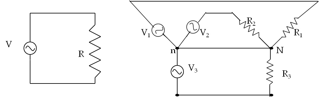
To understand the difference in power fluctuation with time in a one-phase line compared to a three-phase line consider connecting a resistance to each of the voltage sources. As each of the phases in the three-phase line acts independently, we connect each to a separate load in a Y-to-Y connection (Figure 44.1.2). You can look up an advanced book on electric circuits for other ways three-phase lines are connected to circuits. Our objective here is to illustrate power fluctuation in the circuit and a simple Y-to-Y connection will be sufficient. We make a calculation to compare power per load in the two circuits.

Figure 44.1.2. (a) One phase connection across a resistor, and (b) a four-wire Y-to-Y connections for a three-phase circuit. There are other configurations for connecting a three-phase circuits.

Suppose a resistor of resistance \(R\) is connected to each phase of an AC source. What will be the power delivered in the case of a one-phase versus a three-phase source? We have seen in the last chapter that the instantaneous power delivered to a resistor \(R\) in the one-phase line varies with time.

\begin{equation*} P_{\textrm{one-phase}}(t) =\frac{V_0^2}{R} \cos^2(\omega t). \end{equation*}

The instantaneous power delivered to three identical resistors in a three-phase circuit will be independent of time as you can easily verify by expanding the trigonometric functions in the following expression.

\begin{align*} P_{\textrm{three-phase}}(t) \amp =\frac{V_0^2}{R}\left[ \cos^2(\omega t) + \cos^2\left(\omega t+ \frac{2\pi}{3}\right) + \cos^2\left(\omega t+ \frac{4\pi}{3}\right) \right]\\ \amp = \frac{3}{2}\: \frac{V_0^2}{R}. \end{align*}

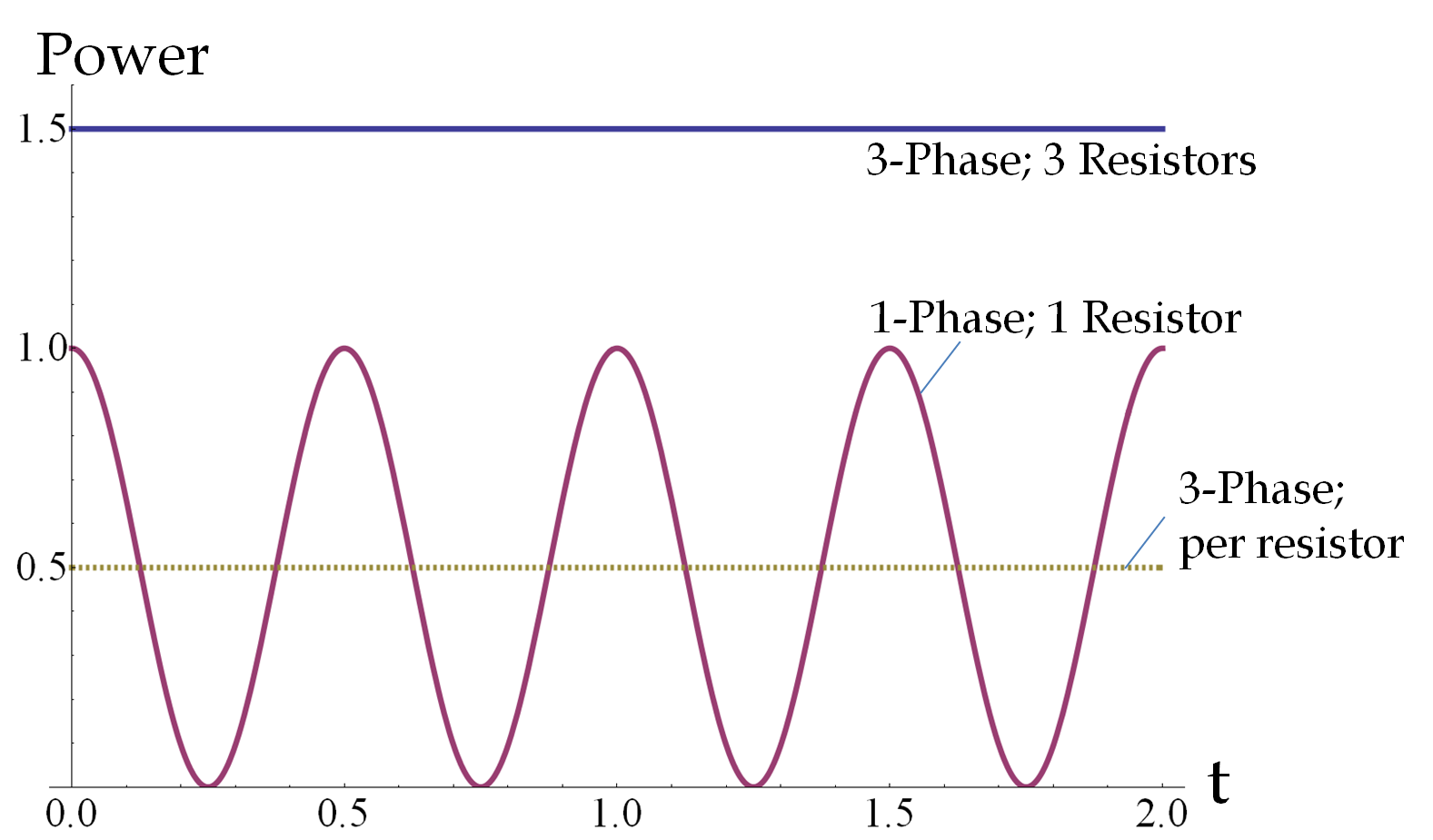
Hence, the total power in a three-phase line is steady as opposed to the pulses in single-phase AC circuits (Figure 44.1.3). This is a great advantage, giving three-phase lines greater stability than identical single-phase line. Nikola Tesla (1856-1943) was the discoverer of polyphase currents who employed two-phase current separated by 90-degree phase. The unit of magnetic field in the SI system of units, viz., \(\text{Tesla}\text{,}\) is named after Nikola Tesla.

Figure 44.1.3. Instantaneous power in an AC circuit using one-phase-one-load versus power in a circuit using a three-phase-three-load line. For these graphs, set \(V_0 = 1\) V, \(R=1\ \Omega\text{,}\) and \(f=1\) Hz. The successive peaks in the one-phase circuit corresponds to the positive and negative cycles of the AC current respectively. The dashed line shows the average power delivered to one resistor, which is the same in the two cases.

Subsection 44.1.2 Phases of Currents and voltages

All currents in the circuit will have the same frequency of oscillation as the driving voltage, but their phases and magnitudes would be different. We will therefore denote each current \(I_a\) by its magnitude \(I_{a0}\) and phase constant \(\phi_a\) for some \(a\text{.}\)

\begin{equation*} I_a = I_{a0}\: \cos(\omega t + \phi_a) \end{equation*}

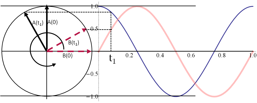
Usually the phase of one of the source voltage will be taken to be the zero-phase reference, and we will then write phases of other quantities relative to this reference. Sometimes we compare two oscillating quantities against one another, and speak of one quantity either leading the other or lagging behind the other. When a current \(I_1\) in the circuit leads another current \(I_2\) in phase, we mean that \(\phi_1-\phi_2\) is positive. In Figure 44.1.4, two sinusoidally oscillating functions whose phase difference or phase shift is \(\pi/2\) rad or \(90^{\circ}\) is illustrated.

Figure 44.1.4. Plot of two oscillating quantities that have a difference of \(\pi/2\) radians in phase. Here functions represented by the phasors are: \(A(t) = \cos(2\pi f t)\) and \(A(t) = \cos(2\pi f t-\pi/2)\text{.}\) The quantity \(A\) leads \(B\text{,}\) or equivalently, \(B\) lags \(A\) as by \(90^{\circ}\) when the phasors rotate in time. The positions of the phasors at \(t=0\) and \(t=t_1\) are indicated in the figure.

In the analysis of an AC-circuit, our task will be to determine the dependence of the magnitude \(I_0\) and phase \(\phi\) of currents in each branch on \(V_0\text{,}\) \(\omega\) and the circuit elements, such as resistance \(R\text{,}\) inductance \(L\) and capacitance \(C\text{.}\)

An AC circuit with only resistors, called a resistive circuit, does not require any special techniques. In the resistive circuits the phases of all currents and voltages are same, and one can carry out the calculations similar to the DC circuits studied in a previous chapter.

But, when there are inductors and/or capacitors present in the circuit, then you must pay close attention to the phases since phases of currents in different branches will, in general be different and phases of voltages across circuit elements will be different. These complications in the calculations for inductive or capacitative circuits make calculations of even simple circuits difficult, as you will see below.

Later in the chapter you will learn an alternative method based on complex algebra that eases the pain a bit, but even there you face tedious algebra. Computer software have also been developed to help analyze complicated circuits.

Subsection 44.1.3 (Calculus) The Ideal AC Generator

AC generator is the ultimate source of all power in the circuit. In an AC generator a sinusoidally varying voltage \(\mathcal{E}(t)\) is generated either by changing the magnetic field with time or moving wires in a magnetic field or both with angular frequency \(\omega\text{,}\) which is related to the frequency \(f\) by \(\omega = 2\pi f\text{.}\)

\begin{equation*} \mathcal{E}(t) = \mathcal{E}_0 \cos(\omega t). \end{equation*}

Since the electric field generated by a changing magnetic field is a non-conservative field, in general, we cannot treat this voltage as a voltage between the two terminals of the AC generator. However, we can think of an “ideal generator” where with some assumptions it would be possible to introduce the concept of voltage for AC generators also.

We will make two assumptions to help us in this regard:

The wires in the generator are perfect conductors.
The magnetic field outside the generator is zero.

By “perfect conductors” we mean that the net force on the conduction electrons is zero. The vanishing of net force on the conduction electrons is necessary for ideal conductors otherwise we would have an infinite acceleration.

The vanishing of the magnetic field outside the generator will imply that the electric field outside the generator will be conservative. This will allow us with the use of potential difference and voltage between points in space, specifically the two terminals of the generator.

Now consider the simple rotating wire generator discussed in the chapter on the Faraday's law. We had found that the voltage induced by the magnetic force on the moving charges in these generators with \(N\) turns is given by

\begin{equation} \mathcal{E}(t) =\omega N A B\cos(\omega t). \label{eq-generator-eqn-emf}\tag{44.1.1} \end{equation}

This must be equal to the line integral of the electric field around a closed path, say aba in Figure 44.1.5, where the segment ab goes through the generator and the segment ba is outside the generator.

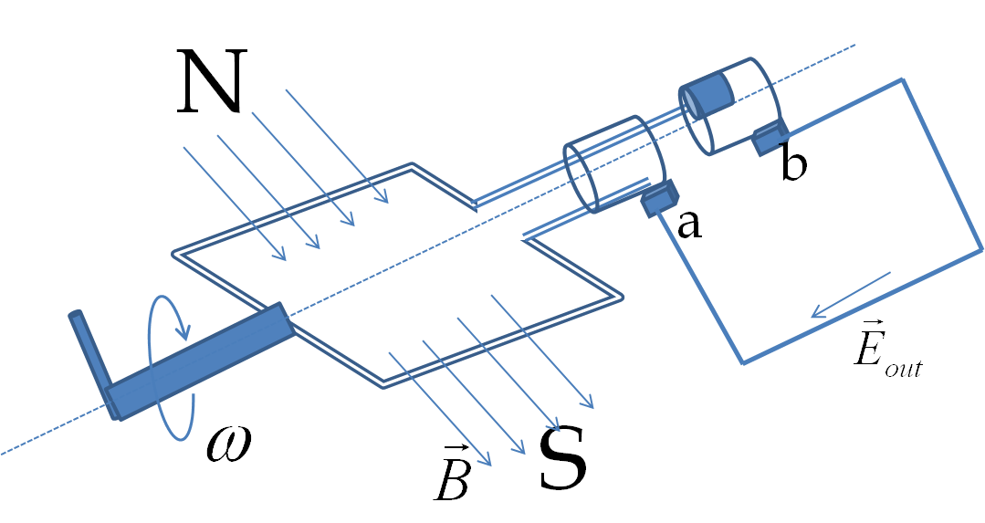
Figure 44.1.5. A generator consisting of a coil that rotates in a magnetic field. The line integral of the electric field is taken from a to b inside the generator and b to a outside. The coil in the generator is assumed to be a perfect conductor and the magnetic field outside is assumed to be negligible. With this assumptions the line integral of the electric field in the loop is equal to the voltage between the terminals a and b.

The line integral of the electric field around this closed loop separates into two parts - one for the inside and the other for the outside.

\begin{equation} \oint \vec E\cdot d\vec l = {\int_{a}^b}_{[\textrm{inside}]} \vec E_{\textrm{in}}\cdot d\vec l + {\int_{b}^a}_{[\textrm{outside}]} \vec E_{\textrm{out}}\cdot d\vec l \label{eq-generator-full-equation}\tag{44.1.2} \end{equation}

First we note that this line integral over the complete loop, the quantity on the left side of this equation, must equal \(-d\Phi_B/dt\) by Faraday's law. Using Eq. (44.1.1), we have

\begin{equation} \oint \vec E\cdot d\vec l = \omega N A B\cos(\omega t).\label{eq-generator-left-side-equation}\tag{44.1.3} \end{equation}

Since we have assumed the wire ab inside the generator to be a perfect conductor, the electric field in them will be zero. Therefore, for the first term on the right side of Eq. (44.1.2) will be zero.

\begin{equation} {\int_{a}^b}_{[\textrm{inside}]} \vec E_{\textrm{in}}\cdot d\vec l = 0 \ \ \textrm{(since perfect conductor)}\tag{44.1.4} \end{equation}

The second term on the right side of Eq. (44.1.2) has segment on the outside of the generator. Since, that part has conservative electric field, the integral will be independent of the path and will depend only upon the end points a and b. The integral will equal to negative of the potential difference \((V_a - V_b)\) between the ends.

\begin{equation*} {\int_{b}^a}_{[\textrm{outside}]} \vec E_{\textrm{out}}\cdot d\vec l = -(V_a - V_b)\ \ \textrm{(since conservative field)}. \end{equation*}

Now, we put all these together to write the final answer for the voltage ate the terminals of the AC generator.

\begin{equation*} V_b - V_a = \omega N A B) \cos(\omega t). \end{equation*}

We can write this as time-dependent voltage \(V(t)\) by absorbing all the constants into one symbol, \(V_0 = \omega N A B\text{.}\)

\begin{equation*} V(t) = V_0 \cos\left(\omega t \right), \end{equation*}

We will call this voltage the AC voltage.