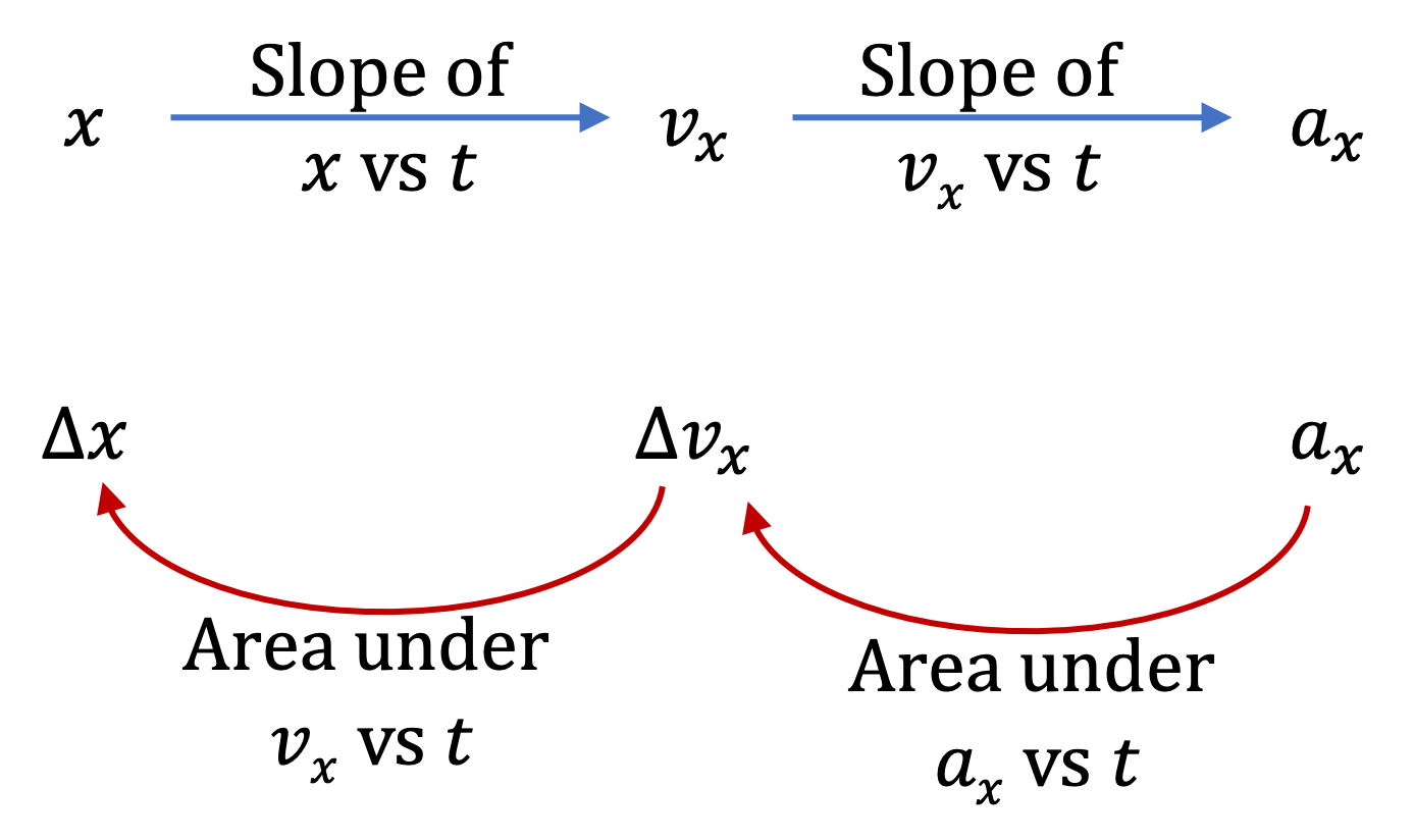
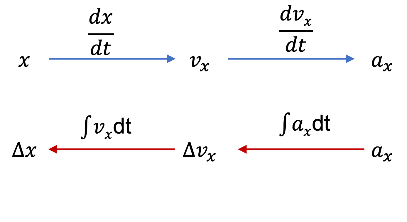
We have covered a lot of ground and it is easy to get overwhelmed. In the end, we are basically studying a simple motion along \(x\)-axis and trying to quantify the rates of change of position \(x \) and velocity \(v_x\text{.}\)Figure 2.55 summarizes how to go from \(x \) to \(v_x\) to \(a_x \text{,}\) and in the reverse order, from \(a_x \) to \(v_x\) to \(x \text{.}\)
Figure2.55.Relations in one-dimensional motion. We compute rate of change from the slopes of tangents of the quantity, and to compute the change in a quantity, we find area under the curve of the rate curve. For instance, to get the rate of change of \(x\text{,}\) i.e., to compute \(v_x\text{,}\) we find the slope of the tangent to the plot of \(x \) versus \(t \text{.}\) This is equivalent to taking the derivative of\(x(t)\text{.}\) Similarly, the rate of change of \(v_x\text{,}\) i.e., \(a_x\) will come from the slope of the tangent to the plot of \(v_x \) versus \(t \text{,}\) which is equivalent to taking the derivative of\(v_x(t)\text{.}\) Going in the reverse order, to compute the change in \(x \) from \(v_x \) versus \(t \) plot, we compute the area under/over the curve, and similarly, to compute the change in \(v_x \) from \(a_x \) versus \(t \) plot, we compute the area under/over the curve of \(a_x\text{.}\) The area under the curve is another way of computing integrals.