Physics Bootcamp

Subsection 21.2.1 Quasi-static Processes

A quasi-static process refers to an idealized or imagined process where the change in state is made infinitesimally slowly so that at each instant the system can be assumed to be in a thermodynamic equilibrium within itself and with the environment.

For instance, imagine heating 1 kg of water from a temperature \(20^{\circ}\text{C}\) to \(21^{\circ}\text{C}\) at a constant pressure of \(1\text{ atm}\text{.}\) To heat the water very slowly we may imagine placing the container with water in a large bath which can be slowly heated such that the temperature of the bath can rise infinitesimally slowly from \(20^{\circ}\text{C}\) to \(21^{\circ}\text{C}\text{.}\) If we put 1 kg water at \(20^{\circ}\text{C}\) directly into a bath which is at \(21^{\circ}\text{C}\text{,}\) the temperature of water will rise rapidly to \(21^{\circ}\text{C}\) in a non-quasi-static way.

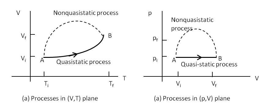
Quasi-static processes are done slowly enough that the system remains at thermodynamic equilibrium at each instant despite the fact that system changes over time. The thermodynamic equilibrium of the system is necessary for the system to have well-defined values of macroscopic properties such as temperature and pressure of the system at each instant of the process. Therefore, quasi-static processes can be shown as well-defined paths in state diagram of the system as shown in Figure 21.2.1. If a finite change occurs fast, we would not know the intermediate states between the initial and final states. Therefore, we display such non-quasistatic processes by dashed curves or lines as shown in the figure.

Since quasi-static process can be analyzed analytically, we will mostly study quasi-static processes in this book. We have already seen that in a quasi-static process, work by a gas is given by \(pdV\text{.}\) Even heat can be written in analytic form if the quasi-static process is also reversible as we will see in the chapter on entropy.

Subsection 21.2.2 Isothermal Process

An isothermal process is a transformation during which temperature of the system is kept fixed. Say, you want to expand a gas at a constant temperature. You can place the gas in a heat-conductive container with a movable piston to heat flow and expansion. Then, you would place the container in a large bath, whose temperature you would maintain by heating or cooling it. You can vary the pressure in the gas by some weights on the piston as illustrated in Figure 21.2.2. Since the piston is freely movable, the pressure inside \(P_{\text{in}}\) is balanced by the pressure outside \(P_{\text{out}}\) by some weights on the piston

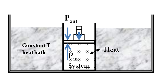
As weights on the piston are removed, an imbalance of forces on the piston develops. The net non-zero force on the piston would cause the piston to accelerate, resulting in an increase in volume. The expansion of the gas cools the gas to a lower temperature, which makes it possible for the heat to enter from the heat bath into the system until the temperature of the gas is reset to the temperature of the heat bath.

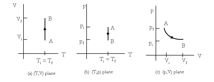
If weights are removed in infinitesimal steps, the pressure in the system will decrease infinitesimally slowly. This way, an isothermal process can be conducted quasi-statically, which we can represent by a line in \((T,p)\text{,}\) \((T,V)\) or \((p,V)\) plane of the gas. On \((T,p)\) and \((T,V) \) diagrams a quasi-static isothermal process will be a straight line perpendicular to the temperature axis, while in the \((p,V) \) diagram, an isothermal is usually a curved line as shown in Figure 21.2.3. For an ideal gas an isothermal process is hyperbolic curve since \(p\sim \frac{1}{V}\) for an ideal gas at constant temperature.

An isothermal process is always conducted quasi-statically, since it to be isothermal throughout the change of volume, you must be able to state the temperature of the system at each step, which is possible only if the system is in thermal equilibrium continuously. Of course, the system must go out of equilibrium for the state to change, but for a quasi-static processes we imagine that the process is conducted in infinitesimal steps such that these departures from equilibrium can be made as brief and as small as we like.

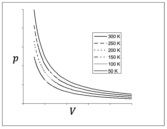
In the \(pV\)-plane different temperatures correspond to different curves. They are called isotherms. In Figure 21.2.4, I have plotted isotherms at various temperatures for an ideal gas by using the ideal gas law, \(pV = nRT = \text{constant}\text{,}\) for an isotherm. Different isotherms correspond to different values of \(T\text{.}\)

Subsection 21.2.3 Isobaric and Isochoric Processes

Besides the isothermal processes, other quasi-static processes of interest for gases are isobaric and isochoric processes. An isobaric process is a process where the pressure of the system does not change while an isochoric process is a process where the volume of the system does not change.

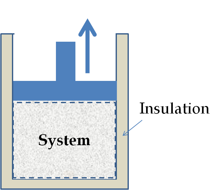
Subsection 21.2.4 Adiabatic Process

In an adiabatic process, the system is thermally insulated from its environment so that no heat is allowed to enter or leave the system. Sometimes, the change is so sudden that there is no time for heat flow. An adiabatic process can be conducted either quasi-statically or nonquasistatically.

In an adiabatic expansion, there are two time scales: rate of the process and the rate at which heat may enter the system through the walls. If the expansion occurs within a time frame in which negligible heat can enter the system, then the process is called adiabatic. Ideally, during an adiabatic process no heat will enter or exit the system.

When a gas expands adiabatically, it must do work against the outside world, and therefore its energy goes down, thus, having the effect of cooling the gas. An adiabatic expansion leads to lowering of temperature and an adiabatic compression to the increase of temperature. Adiabatic expansion is one mechanism by which gases are liquefied.