
Section 43.2 Damping by Resistance

There is no resistance in the ideal LC circuit in which even the resistance in teh wires is ignored. In reality, however, there is always some resistance in the circuit, for instance in the connecting wires and the materials of the inductor and the capacitor, which dissipate energy. Dissipation of energy from the circuit results in a decrease in current over time.

Oscillatory circuits also radiate electromagnetic waves and lose energy through radiation. We will not discuss the radiation of energy now, and assume that the loss by radiation is negligible compared to the loss due to resistance.

To understand the phenomenon of resistive damping better consider a circuit with a resistor \(R\) in series with a capacitor \(C\) and an inductor \(L\) as shown in Figure 43.2.1.

Let the capacitor be charged initially with charges \(\pm Q_0\) on the plates so that there is a voltage \(V_0 = Q_0/C\) at time \(t=0\) between the capacitor plates.

Figure 43.2.1.

When the switch is closed at \(t=0\text{,}\) current in the circuit will rise from zero to a maximum value, and then, depending on the values of \(R/2L\) vs \(1/\sqrt{LC} \text{,}\) current will oscillate with decreasing amplitude or simply damp out as illustrated in Figure 43.2.2 below. Three types of behavior are seen.

  1. Underdamped Case. If \(R/2L \lt 1/\sqrt{LC}\text{,}\) then current in the circuit oscillates about the equilibrium value of zero, successively damping out each cycle.
  2. Over-damped Case. If \(R/2L \gt 1/\sqrt{LC}\text{,}\) then current in the circuit does not oscillate; current just damps out to zero.
  3. Critically Damped Case. If \(R/2L = 1/\sqrt{LC}\text{,}\) then current in the circuit does not oscillate; current just damps out to zero rather quickly.

These three types of behavior of the circuit are more compactly presented by using the following combination of constants.

\begin{align} \amp \omega_0 = \dfrac{1}{\sqrt{LC}},\ \ \ \gamma = \dfrac{R}{L}\tag{43.2.1}\\ \amp \omega_1 = \sqrt{ \omega_0^2 - \gamma^2/4 },\ \ \ \alpha = \sqrt{ \gamma^2/4 - \omega_0^2 }\tag{43.2.2} \end{align}

For underdapmed \(\omega_1\) is the angular frequency of oscillations and \(\omega_0\) is the angular frequency when there is no damping. Sometimes \(\omega_0\) is also called natural frequency. Constant \(\gamma\) is called the damping parameter. Constant \(\alpha \) is a positive real number in overdamped case.

After solving Eq. (43.2.9) for \(q\text{,}\) derived for the RLC-circuit below, we can get current by \(I=dq/dt\text{.}\) We find that current \(I(t)\) at time \(t\) with zero current at \(t=0\) and charge \(\pm Q_0\) at capacitor plates at \(t=0\) for underdamped, overdamped, and critically-damped cases are given by the following expression.

\begin{align} I \amp = \begin{cases} I_u = -Q_0\,e^{-\gamma\,t/2}\left( \dfrac{\gamma^2 + 4\omega_1^2}{4\omega_1} \right)\,\sin(\omega_1 t), \amp \omega_0 \gt \gamma/2,\\ I_o = -\alpha\,Q_0 \left( 1-\dfrac{\gamma^2}{4\alpha^2} \right) \,e^{-\gamma\,t/2}\sinh(\alpha t), \amp \omega_0 \lt \gamma/2,\\ I_c = -\dfrac{\gamma^2}{4} Q_0\,t\,e^{-\gamma\,t/2}, \amp \omega_0 = \gamma/2, \end{cases}\notag\\ \amp \label{eq-currents-in-damped-circuit}\tag{43.2.3} \end{align}

where \(I_u\text{,}\) \(I_o\text{,}\) and \(I_c\) refer to underdamped, overdamped, and critically-damped cases, and \(\sinh(x)\) is the sinh function whose explicit representation in terms of exponetials is

\begin{equation*} \sinh(x) = \dfrac{e^{x} - e^{-x}}{2}. \end{equation*}

Figure 43.2.2 displays current in three types of damping. Critical damping id preferred over overdamping when you need to damp current quickly. Underdamping is important when studying oscillatory circuits, such as AC circuit and antennas.

Figure 43.2.2. Three types of damping illustrated. Parameters used for plot: (1) Underdamped \(R = 0.25\,\Omega\text{,}\) \(C=1\text{ F}\text{,}\) \(L = 1\text{ H}\text{,}\) (2) Overdamped \(R = 4\,\Omega\text{,}\) \(C=1\text{ F}\text{,}\) \(L = 1\text{ H}\text{,}\) (3) Critically damped \(R = 2\,\Omega\text{,}\) \(C=1\text{ F}\text{,}\) \(L = 1\text{ H}\text{.}\) The initial state: \(q(0) = Q_0\) and \(I(0)=0\text{.}\)

Subsection 43.2.1 Meaning of \(\gamma\)

To gain an understanding of the meaning of the damping parameter \(\gamma\) we look at underdamped oscillatory circuit. You will notice that the envelop of oscillations, i.e., the plot that has peaks or troughs as their points, falls off with time exponentially. The time for peak current to fall off to a fraction \(\dfrac{1}{e}\) of its max at some time is equal to \(2/\gamma\) as illustrated in Figure 43.2.3.

Figure 43.2.3. Envelops of an underdamped oscillations illustrate the time for current in the envelop to drop to \(1/e\) of the initial value is \(2/\gamma\text{.}\) Parameters used for plot: \(R = 0.25\,\Omega\text{,}\) \(C=1\text{ F}\text{,}\) \(L = 1\text{ H}\text{.}\) The initial state: \(q(0) = Q_0\) and \(I(0)=0\text{.}\)

The energy of the circuit is given by

\begin{equation*} U_\text{circuit} = \frac{1}{2}LI^2 + \frac{1}{2}CV_C^2. \end{equation*}

This also oscillates and decays with time. Its envelop drops twice as fast as that shown in Figure 43.2.3 for the current. The time taken for energy envelop to drop by \(1/e\) is equal to \(1/\gamma\text{.}\) This is called time constant of the circuit.

Subsection 43.2.2 Quality Factor Q of an Oscillator

Quality factor provides a standard way to talk about goodness of an oscillator. We denote Quality factor by \(Q\text{.}\) A simple measure of Quality of an oscillator would be to divide the average energy in a particular cycle by the energy lost in the cycle, so that the less the energy is lost in a cycle, the more persistent are the oscillations, and therefore, higher the Quality.

For technical reasons, we define \(Q \) factor by dividing the energy at the beginning of a cycle to the energy lost in \(\dfrac{1}{2\pi}\) of a cycle. The factor is not critical to the definition, but does give simpler formula when we apply this to a lightly damped oscillator. Suppose \(U(t)\) be the energy at time \(t\text{,}\) then we would compute \(Q\) by

\begin{equation} Q = \dfrac{U(t)}{\left| \Delta U\left(\text{during }t\text{ to }t+ \dfrac{1}{\omega}\right) \right| };.\tag{43.2.4} \end{equation}

We get a simple formula for \(Q\) when oscillator is a good oscillator, for instance, when

\begin{equation} \gamma \lt\lt \omega_0.\tag{43.2.5} \end{equation}

Under these conditions, the oscillator is called a lightly damped oscillator. For lightly damped case, energy envelop decreases exponentially and is given by

\begin{equation} U(t) = U(0) e^{-\gamma t}.\tag{43.2.6} \end{equation}

It is then easy to work out energy lost during interval from \(t=t\) to \(t=t + \dfrac{1}{\omega} \text{.}\) The quality factor obtained by this calculation is

\begin{equation} Q = \dfrac{\omega_0}{\gamma} = \dfrac{\sqrt{L}}{R\sqrt{C}}\ \ \ \ \ (\text{lightly damped oscillator})\tag{43.2.7} \end{equation}

Often, we use this formula, even when the underdamped oscillator is not lightly damped. In those cases, we just replace \(\omega \) in this formula by \(\omega_1\text{,}\) the actual angular frequency of the damped oscillator.

\begin{equation} Q \sim \dfrac{\omega_1}{\gamma}\ \ \ \ \ (\text{underdamped oscillators})\tag{43.2.8} \end{equation}

Good mechanical oscillators such as tuning forks and guitar strings have \(Q\) values in the thousands. Laser cavities, which are electromagnetic wave oscillators, have much higher \(Q\) values, exceeding \(10^7\text{.}\) Of course, the undamped oscillator has zero \(\gamma\text{,}\) and hence infinite \(Q\text{.}\) There is no \(Q\) for the critically damped and overdamped cases since they do not oscillate. You might say, their \(Q = 0\text{.}\)

Subsection 43.2.3 (Calculus) Equation of Motion of RLC circuit

Faraday's flux rule around the circuit of Figure 43.2.4 gives rise to a second order differential equation for charge \(q(t)\) on the positive plate of the capacitor.

Let \(\mathcal{E}_L\text{,}\) \(\mathcal{E}_R\text{,}\) and \(\mathcal{E}_C\) be EMF's around inductor, capacitor, and resistor, respectively. These are

\begin{equation*} \mathcal{E}_L = L\frac{dI}{dt},\ \ \mathcal{E}_R = IR,\ \ \mathcal{E}_C=\frac{1}{C}\,q, \end{equation*}

with \(I = dq/dt\text{.}\)

Figure 43.2.4.

Going around the circuit loop, we get

\begin{equation*} \mathcal{E}_L + \mathcal{E}_R + \mathcal{E}_C =0. \end{equation*}

In terms of \(q(t)\text{,}\) the charge on positive plate of the capacior at instant \(t\text{,}\) this is

\begin{equation} L\frac{d^2q}{dt^2} + R\frac{dq}{dt} + \frac{1}{C}\,q=0.\label{eq-motion-of-q-in-damped-circuit-diff-eq}\tag{43.2.9} \end{equation}

Subsection 43.2.4 (Calculus) Solution of Equation of Motion of RLC circuit

The solution of Eq. (43.2.9) depends on relative values of \(R/L\) and \(1/\sqrt{LC}\text{.}\) We denote these quantites by other symbols.

\begin{equation*} \omega_0 = \dfrac{1}{\sqrt{LC}},\ \ \gamma = \dfrac{R}{L}. \end{equation*}

With these changes Eq. (43.2.9) becomes

\begin{equation*} \dfrac{d^2 q}{d t^2} + \gamma\, \dfrac{dq}{dt} + \omega_0^2\, q = 0. \end{equation*}

Let us make the following substitution.

\begin{equation} q(t) = e^{-\gamma\,t/2}\, x(t).\label{eq-motion-q-x-relation}\tag{43.2.10} \end{equation}

With this we get

\begin{equation} \dfrac{d^2 x}{d t^2} + \left( \omega_0^2 - \gamma^2/4 \right) x = 0\label{eq-motion-of-x}\tag{43.2.11} \end{equation}

The solution of this equation depends on \(\left( \omega_0^2 - \gamma^2/4 \right)\text{.}\) If this constant is positive, we will have \(x\) as sine and cosine functions, if negative, the solution will be exponetial function, and if zero, \(x\) will be linear in \(t\text{.}\)

\begin{align} x \amp = \begin{cases} x_u = A\, \cos(\omega_1 t) + B\, \sin(\omega_1 t), \ \ \omega_1^2 = \omega_0^2 - \gamma^2/4 \gt 0,\\ x_o = A\, e^{\alpha t} + B\, e^{-\alpha t}, \ \ \alpha^2 = \gamma^2/4 - \omega_0^2 \gt 0,\\ x_c = A + B\,t, \ \ \omega_0 = \gamma/2 \end{cases}\notag\\ \amp \label{solution-x-with-contants}\tag{43.2.12} \end{align}

These three cases correspond to underdampig, overdamping, and critical damping respectively. Using these answers for \(x\) in Eq. (43.2.10) gives us general solution. Note, in general solution we have two unknown constants \(A \) and \(B\text{.}\) We fix these constants from values of the initial charge \(q(0)\) and initial current \(I(0)\text{.}\)

Subsubsection 43.2.4.1 Underdamping Case with \(q(0)=Q_0\) and \(I(0)=0\)

We now show how we can fix two undetermined constants in general solutions in Eq. (43.2.12). To be specific, we will work out the details for only the underdamped case.

We start with general solutions for \(q(t)\) and \(I(t)\text{.}\)

\begin{align*} \amp q(t) = e^{-\gamma\,t/2} \left( A\, \cos(\omega_1 t) + B\, \sin(\omega_1 t) \right), \\ \amp I(t) = \dfrac{d q(t)}{dt} = -\dfrac{\gamma}{2} q(t) + \omega_1\,e^{-\gamma\,t/2} \left(- A\, \sin(\omega_1 t) + B\, \cos(\omega_1 t) \right). \end{align*}

Now, we set \(t=0\) in them and use the initial values.

\begin{align*} \amp Q_0 = A, \\ \amp 0 = -\dfrac{\gamma}{2} Q_0 + \omega_1\, B. \end{align*}

Therefore we have the charge and current at arbitrary time

\begin{align*} \amp q(t) = Q_0\,e^{-\gamma\,t/2} \left[\cos(\omega_1 t) + \dfrac{\gamma}{2\omega_1}\,\sin(\omega_1 t) \right], \\ \amp I(t) = - Q_0\, \left( \omega_1 + \dfrac{\gamma^2}{4\omega_1} \right) \,e^{-\gamma\,t/2} \sin(\omega_1 t). \end{align*}

You can try to find solutions for other initial conditions and for the other two damping cases.

Consider RLC-circuit shown in Figure 43.2.6 and answer the following questions. (a) Find the natural frequency \(\omega_0\) and the damping parameter \(\gamma\text{,}\) and determine if the circuit is under-damped, over-damped or critically damped.

Figure 43.2.6.

(b) At \(t=0\text{,}\) the charge on the capacitor was 15 \(\mu\)C and the current in the circuit was zero, find the current in the circuit at an arbitrary time.

(c) What is the \(Q\) factor of the oscillator?

(d) (Calculus) How much energy is dissipated in first 2 seconds?

Hint

(a) Use defining equations, (b) USe \(I_u\text{,}\) (c) Integrate power, \(I^2R\text{.}\)

Answer

(a) \(2887\ \text{sec}^{-1} \text{,}\) \(3334\ \text{sec}^{-1}\text{,}\) underdamped, (b) \(-53\text{ mA}\, e^{-1667\,t}\,\sin(2357\, t)\text{,}\) (c) \(0.7\text{,}\) (d) \(2.8\:\mu\text{J}\text{.}\)

Solution 1 (a)

(a) The natural frequency,

\begin{equation*} \omega_0 =\frac{1}{\sqrt{LC}} = \frac{1}{\sqrt{3\times10^{-3}\:\text{H}\times40\times10^{-6}\:\text{F}}} = 2887\ \text{sec}^{-1} \end{equation*}

The damping parameter,

\begin{equation*} \gamma = \frac{R}{L} = \frac{10\ \Omega}{3\times 10^{-3}\:\text{H}} = 3334\ \text{sec}^{-1}. \end{equation*}

Since \(\omega_0>\gamma/2\text{,}\) the circuit is under-damped.

Solution 2 (b)

(b) Putting in the numbers in \(I_u\) in Eq. (43.2.3), we obtain the following for the current in the circuit with \(t\) in sec. We will find the multiplying factor in the equation separately.

\begin{equation*} \omega_1 = \sqrt{ \omega_0^2 - \gamma^2/4 } = 2357\text{ sec}^{-1}. \end{equation*}

This gives the following for the factor in the solution.

\begin{align*} \text{factor}\amp = \left( \dfrac{\gamma^2 + 4\omega_1^2}{4\omega_1} \right)\\ \amp = \left( \dfrac{3334^2 + 4\times 2357^2}{4 \times 2357} \right) = 3536\text{ sec}^{-1}. \end{align*}

Finally, using the formula for \(I_u\) we get

\begin{align*} I \amp = -Q_0\,\left( \dfrac{\gamma^2 + 4\omega_1^2}{4\omega_1} \right)\, e^{-\gamma\,t/2}\,\sin(\omega_1 t),\\ \amp = -15\,\mu\text{C}\times 3536\text{ s}^{-1}\, e^{-1667\,t}\,\sin(2357\, t),\\ \amp = -53\text{ mA}\, e^{-1667\,t}\,\sin(2357\, t). \end{align*}
Solution 3 (c)

(c) We will use \(\omega_1\) for the \(Q\) factor.

\begin{align*} Q\amp = \dfrac{\omega_1}{\gamma} = \dfrac{2357}{3334} = 0.7. \end{align*}

If you use \(\omega_0\) in place of \(\omega_1\text{,}\) you will get a little larger value, here you will get \(0.9\text{.}\) They are both order, \(O(1)\text{,}\) i.e., the oscillator is not very good. If you get a \(Q\) of \(10\) or more, you will have a very good oscillator.

Solution 4 (d)

(d) Integrate power deposited in duration (0, 2 sec) by inserting \(I(t)\) in part (b).

\begin{equation*} \text{Energy} = \int_0^2 I^2\: R dt = 2.8\:\mu\text{J}. \end{equation*}

Determine if the circuits in Figure 43.2.8 are under-damped, over-damped, or critically damped.
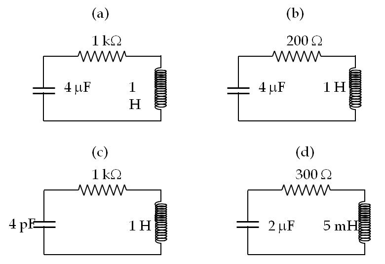
Figure 43.2.8. For Checkpoint 43.2.7.
Hint

Compare \(\omega_0\) to \(\gamma/2\text{.}\)

Answer

(a) critically damped, (b) under-damped, (c) under-damped, (d) over-damped.

Solution 1 (a)

We will use damping parameter \(\beta = \gamma/2\) rather than \(\gamma\text{.}\) It will simplify notation.

(a) The parameters of the given circuit are

\begin{align*} \amp \beta = \dfrac{R}{2L} = \dfrac{1000\:\Omega}{2\times 1\:\text{H}} = 500\:\text{sec}^{-1},\\ \amp \omega_0 = \dfrac{1}{\sqrt{LC}} = \dfrac{1}{\sqrt{1\:\text{H}\times 4\times 10^{-6}\:\text{F}}} = 500\:\text{sec}^{-1}. \end{align*}

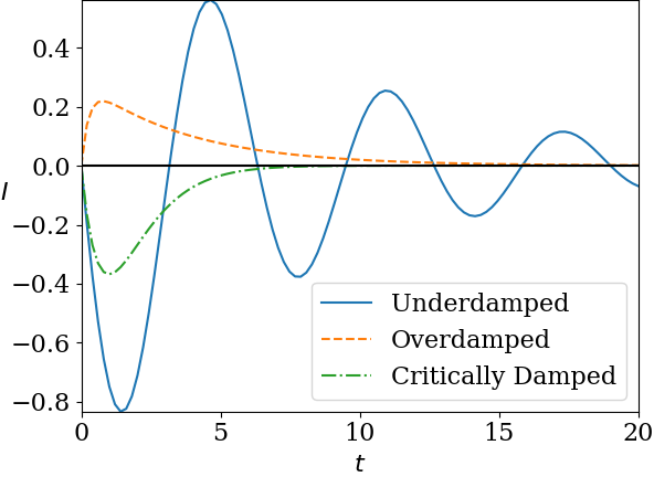
Since \(\omega_0 = \beta\text{,}\) this circuit is critically damped.

Solution 2 (b)

We will use damping parameter \(\beta = \gamma/2\) rather than \(\gamma\text{.}\) It will simplify notation.

(b) The parameters of the given circuit are

\begin{align*} \amp \beta = \dfrac{R}{2L} = \dfrac{200\:\Omega}{2\times 1\:\text{H}} = 100\:\text{sec}^{-1},\\ \amp \omega_0 = \dfrac{1}{\sqrt{LC}} = \dfrac{1}{\sqrt{1\:\text{H}\times 4\times 10^{-6}\:\text{F}}} = 500\:\text{sec}^{-1}. \end{align*}

Since \(\omega_0 \gt \beta\text{,}\) this circuit is under-damped.

Solution 3 (c)

We will use damping parameter \(\beta = \gamma/2\) rather than \(\gamma\text{.}\) It will simplify notation.

(c) The parameters of the given circuit are

\begin{align*} \amp \beta = \dfrac{R}{2L} = \dfrac{1000\:\Omega}{2\times 1\:\text{H}} = 500\:\text{sec}^{-1},\\ \amp \omega_0 = \dfrac{1}{\sqrt{LC}} = \dfrac{1}{\sqrt{1\:\text{H}\times 4\times 10^{-12}\:\text{F}}} = 500,000\:\text{sec}^{-1}. \end{align*}

Since \(\omega_0 > \beta\text{,}\) this circuit is under-damped.

Solution 4 (d)

We will use damping parameter \(\beta = \gamma/2\) rather than \(\gamma\text{.}\) It will simplify notation.

(d) The parameters of the given circuit are

\begin{align*} \amp \beta = \dfrac{R}{2L} = \dfrac{300\:\Omega}{2\times 5\times 10^{-3}\:\text{H}} = 30,000\:\text{sec}^{-1},\\ \amp \omega_0 = \dfrac{1}{\sqrt{LC}} = \dfrac{1}{\sqrt{5\times 10^{-3}\:\text{H}\times 2\times 10^{-6}\:\text{F}}} = 10,000\:\text{sec}^{-1}. \end{align*}

Since \(\omega_0 \lt \beta\text{,}\) this circuit is over-damped.