We have seen in previous sections that mechanics of two-body system interacting via a gravitational force is best done in the CM frame, where it suffices to work out the equivalent problem of the orbit of a fictitious particle with mass equal to the reduced mass and center of mass kept at rest at the origin. Once, we solve this equivalent problem of the orbit of the fictitious particle, we can immediately work out the orbits of two masses by utilizing the relation between the coordinates of the reduced mass and the coordinates of the individual masses as we have already discussed.
Furthermore, a two-body system interacting via a gravitational force, it is sufficient to examine the conservation of angular momentum and the conservation of energy in the system. As above, let us denote the conserved angular momentum by \(l\) and conserved energy by \(E\) and work with polar coordinates \(r\) and \(\theta\) in the plane perpendicular to the direction of the constant angular momentum vector.
\begin{align}
\amp \mu r^2 \dfrac{d\theta}{dt} = l,\tag{12.55}\\
\amp \dfrac{1}{2}\mu\left( \dfrac{dr}{dt} \right)^2 + U_\text{eff}(r) = E.\tag{12.56}\\
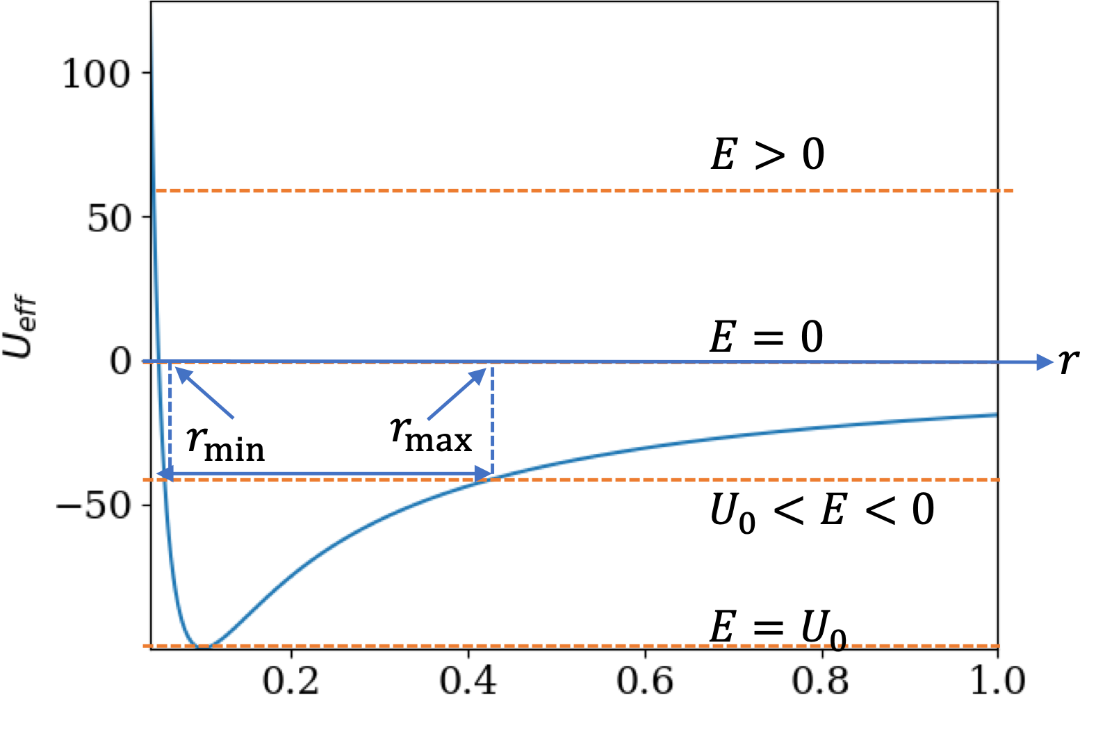
\amp U_\text{eff}(r) = \frac{1}{2}\frac{l^2}{\mu r^2} - \frac{G_N m_1 m_2}{r}\tag{12.57}
\end{align}
To get trajectory of \(\mu\) in the two-dimensional plane from these equations, we can deduce the equation obeyed by \(dr/d\theta\) and try to integrate that.
\begin{equation}
\frac{dr}{d\theta} = \pm \frac{\sqrt{2\mu}}{l}\,r^2\,\sqrt{E - U_\text{eff}(r)}\tag{12.58}
\end{equation}
This task is simplified if we redefine radial and energy in terms of natural scales in this problem, which has the added benefit of absorbing the constants into one overall symbol. We use the minimum of the effective potential energy for scaling purposes. That minimum provides us with a length scale and an energy scale. From \(dU_\text{eff} = 0\text{,}\) we get
\begin{align*}
\amp r_0 = \frac{2\alpha}{\beta} = \frac{l^2}{G_N m_1 m_2 \mu}\\
\amp U_0 \equiv U_\text{eff,min} = -\frac{-\beta^2}{4\alpha} = \frac{G_N^2 m_1^2 m_2^2 \mu}{2 l^2}.
\end{align*}
Now, we intruduce the following scaled quantities
\begin{align}
\amp \rho = \frac{r}{r_0}\tag{12.59}\\
\amp \epsilon = \frac{E}{|U_0|} \tag{12.60}
\end{align}
Try to set
\(r = r_0\,\rho\) and
\(E = |U_0|\,\epsilon\) in
(12.58) and perform all the algebra to arrive at
\begin{equation}
\frac{d\rho}{d\theta} = \pm \rho^2\,\sqrt{\epsilon^2 - \frac{1}{\rho^2} + \frac{2}{\rho} }. \tag{12.61}
\end{equation}
This can be integrated to give
\begin{equation*}
\int_{\theta_\text{ref}}^\theta\,d\theta = \pm \int_{\rho_\text{ref}}^{\rho} \frac{d\rho}{\rho^2\sqrt{\epsilon - (1/\rho^2) + (2/\rho) }},
\end{equation*}
where (\(\rho_\text{ref}, \theta_\text{ref}\)) are arbitrary point in the two-dimensional plane. You can look up an integral table to do the integral on the right side. Or, do a couple of substitutions: (1) \(u=1/\rho\text{,}\) (2) \(v-u-1\text{,}\) (3) \(w = v/\sqrt{\epsilon + 1}\text{,}\) (4) \(w = \cos\phi\text{.}\) And, then substitute back. Answer will be
\begin{equation*}
\theta - \theta_\text{ref} = \cos^{-1}\left( \frac{(1/\rho) - 1}{ \sqrt{\epsilon + 1}} \right) - \cos^{-1}\left( \frac{(1/\rho_\text{ref}) - 1}{ \sqrt{\epsilon + 1}} \right)
\end{equation*}
Now, since \(\theta_\text{ref}\) was arbitrary to begin with, we can choose a value that simplifies the formula. Let’s choose
\begin{equation*}
\theta_\text{ref} = \cos^{-1}\left( \frac{(1/\rho_\text{ref}) - 1}{ \sqrt{\epsilon + 1}} \right).
\end{equation*}
Then, the relation between scaled radial coordinate \(\rho\) and \(\theta\) will be
\begin{equation*}
\cos\theta = \frac{(1/\rho) - 1}{ \sqrt{\epsilon + 1}}.
\end{equation*}
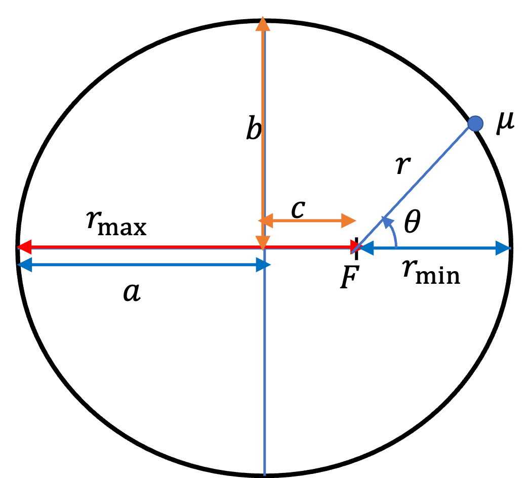
Rearranging and setting \(e= \sqrt{\epsilon + 1}\) we see that it the the orbit equation presented above.
\begin{equation*}
\rho = \frac{1}{1 + e \cos\theta},
\end{equation*}
Now, we replace the scaled radial variable \(\rho\) by \(r/r_0\text{,}\) where \(r_0\) is the minimum of the effective potential to get the orbit equation give above.
\begin{equation*}
r = \frac{r_0}{1 + e \cos\theta},
\end{equation*}