
Section 39.4 Ampere's Law

Ampere's law states that circulation of magnetic field around a loop is proportional to net current passing through the area within the loop, which we call enclosed current and denote it by \(I_\text{enc}\text{.}\) Specifically,

\begin{equation} \text{Circulation of the } \vec B \text{ field} = \mu_0\, I_\text{enc}.\label{eq-amperes-law-non-calculus}\tag{39.4.1} \end{equation}

In Calculus language, this is

\begin{equation} \oint_C\, \vec B\cdot d\vec l = \mu_0\, I_\text{enc},\label{eq-amperes-law-calculus}\tag{39.4.2} \end{equation}

where \(C\) is the directed closed path over which the line integral is to be performed. On the right side, the enclosed current can be postive or negative depending on the direction of current as it relates to the direction of loop C. The direction of positive current and loop C are illustrated in Figure 39.4.1. Note that direction of loop C may or may not be the same as the direction of magnetic field - loop is picked independently of the magnetic field.

A particular emclosed current is positive or negative when included to get the net enclosed current as illustrated in Figure 39.4.1. When you apply right-hand rule on the direction of the loop, by sweeping your right palm around the loop and positive current in the direction of the thumb; the opposite direction to the thumb is treated as negative.

Figure 39.4.1. Positive current versus loop direction.

\(I_\text{enc}\) is the net of all positive and negative currents. Figure 39.4.2 illustrates Ampere's law for a number of loops.

The loop over which we compute circulation for use in Ampere's law is called the Amperial loop. This loop is a loop in space and no physical structure, such as wire or anything else need be present at points of the loop. Sometimes we refer to these loops as loops in space or mathematical loop.

Figure 39.4.2. The value of circulation of magnetic field around Amperian loops can be stated immediately if we know the amount of current enclosed by the loop and the direction from the right-hand-rule applied to the direction of the loop; we do not need to know magnetic field or calculate the circulation integral. In this figure, using Ampere's law we can state that circulation through loop \(\text{L}_1\) and \(\text{L}_2\) are same, both equal to \(\mu_0 I\text{,}\) circulation through \(\text{L}_3\) is \(-\mu_0 I\text{,}\) which is negative since current through the loop is in the opposite direction of loop, circulation through \(\text{L}_4\) is zero since it has oppositely directed current through the loop which add up to zero, and circulation through \(\text{L}_5\) is zero since no current passes through the loop.

Subsection 39.4.1 (Calculus) Strategy for Using Ampere's Law

How can we use Ampere's law to find magnetic field? The statement of Ampere's law given in Eq. (39.4.2) shows that the unknown magnetic field is part of the integrand. Therefore, we can use Ampere's law to calculate magnetic field only in those situations when magnetic field can come out of the integrand.

So, when can \(B\) can come out of integrand of the circulation integral? It turns out that Biot-Savart law (Subsection 39.1.1) helps us make general statements about magnetic field in the case of the three symmetric situations discussed below.

Using Biot-Savart law, it is possible to state direction and distance-dependence functional form of magnetic field, even though calculating the exact formula may be difficult. Once we have these informations, we can choose Amperian loop accordingly, such that on the path chosen, \(\vec B\cdot d\vec l\) is either zero or some constant mgnitude \(B\) times a length.

The three special symmetries that allow these special Amperian loops are

  1. Cylindrical symmetry. This is the case when current is along a long straight wire. Here Amperian loop will be a circle.
  2. Planar symmetry. This is the case if current is on a flat large surface. Here, Amperian loop is a rectangle perpendicular to the surface and passes through the surface.
  3. Solenoidal symmetry. This is the case if current is along \(\hat u_{\phi}\) of cylindrical coordinate. A cylinder that has an insulated wires wound on a cylinder has solenoidal symmetry if the cylinder is long and the area of cross-section is small. Here, Amperian loop is a rectangle that has one side inside and one side outside and runs parallel to the cylinder.

Subsection 39.4.2 (Calculus) Steps in Solving Ampere's Law Problems

When applying Ampere's law to find a formula for the magnetic field, we treat \(\vec B\) in the following equation to be the unknown.

\begin{equation*} \oint_{C}\, \vec B\cdot d\vec l = \mu_0 I_\text{encl}. \end{equation*}

Immediately, you should notice that we need to somehow know the closed path \(C\) we will use, and somehow find \(I_\text{enc}\text{.}\) We follow the following four-step process. Notice that calculation is step is way down in the fourth step - without an understanding of steps 1, 2, and 3, just doing calculations is not possible.

  1. Direction of \(\vec B\text{:}\) Using Biot-Savart right-hand rule, guess the direction of \(\vec B\)
  2. Functional form of \(B\text{:}\) Using symmetry guess the functional dependence of magnitude \(B(x,y,z)\text{,}\) i.e., answer the following types of questions: is it a function of \(x\) only, is it a function of \(s=\sqrt{x^2 + y^2}\) only , is it a function of only \(z\text{,}\) etc.
  3. Choosing Amperian Loop: Using the information gathered, we imagine a closed loop, the Amperian loop, that has the following characteristics:

    1. Cantain the field point: The Amperian loop passes through the field point of interest,
    2. Direction of \(\vec B\) versus direction of loop: \(\vec B\) at every point of the loop is either parallel or antiparallel or perpendicular to the loop direction at that point,
    3. \(B\) be a multiple of \(B_P\text{:}\) Magnitdue \(B\) at the field point, \(B_P\) is same either everywhere on the Amperian loop or at finite segments of the loop. In the case of \(B\) not same at all points of the Amperian loop, we require that \(B\) be a multiple of the value at the field points - the mutiplying factor can be zero.
  4. Calculations:

    1. Circulation: With Amperian loop chosen, the left side of Ampere's law turns into a simple product, which can be written as a product of magnitude \(B_P\) and a length \(L\text{,}\) which will have characteristics of the Amperian loop chosen.
      \begin{equation*} \text{Left Side } = B_P L. \end{equation*}
    2. \(I_\text{enc}\text{:}\) The right side is computed either directly from the diagram and noting currents crossing the area or by integrating some current density over appropriate cross-section, as you have learned in the chapter on electric currents. For volume current density, \(\vec J\text{,}\) you would integrate over the area of cross-section and for the surface current density, \(\vec K\text{,}\) you will integrate over the line of cross-section.
    3. Solve: In all cases, we will get an equation of the following form when we apply Ampere's law.
      \begin{equation*} B_P L = \mu_0 I_\text{enc}, \end{equation*}
      which immediately gives the magnitude of the field to be
      \begin{equation*} B_P = \dfrac{\mu_0 I_\text{enc}}{L}. \end{equation*}

As a first example of application of Ampere's law for finding magnetic field, we will find the magnetic field at a distance \(s\) from a current \(I\) in infintely long wire. We already know the answer to this problem by applying Biot-Savart Law, but we will re-do this case to explicitly lay out arguments common to all applications of Ampere's law. Just to recall the answer.

\begin{align*} \amp \text{Magnitude, } B = \dfrac{\mu_0}{2\pi}\,\dfrac{I}{s}.\\ 
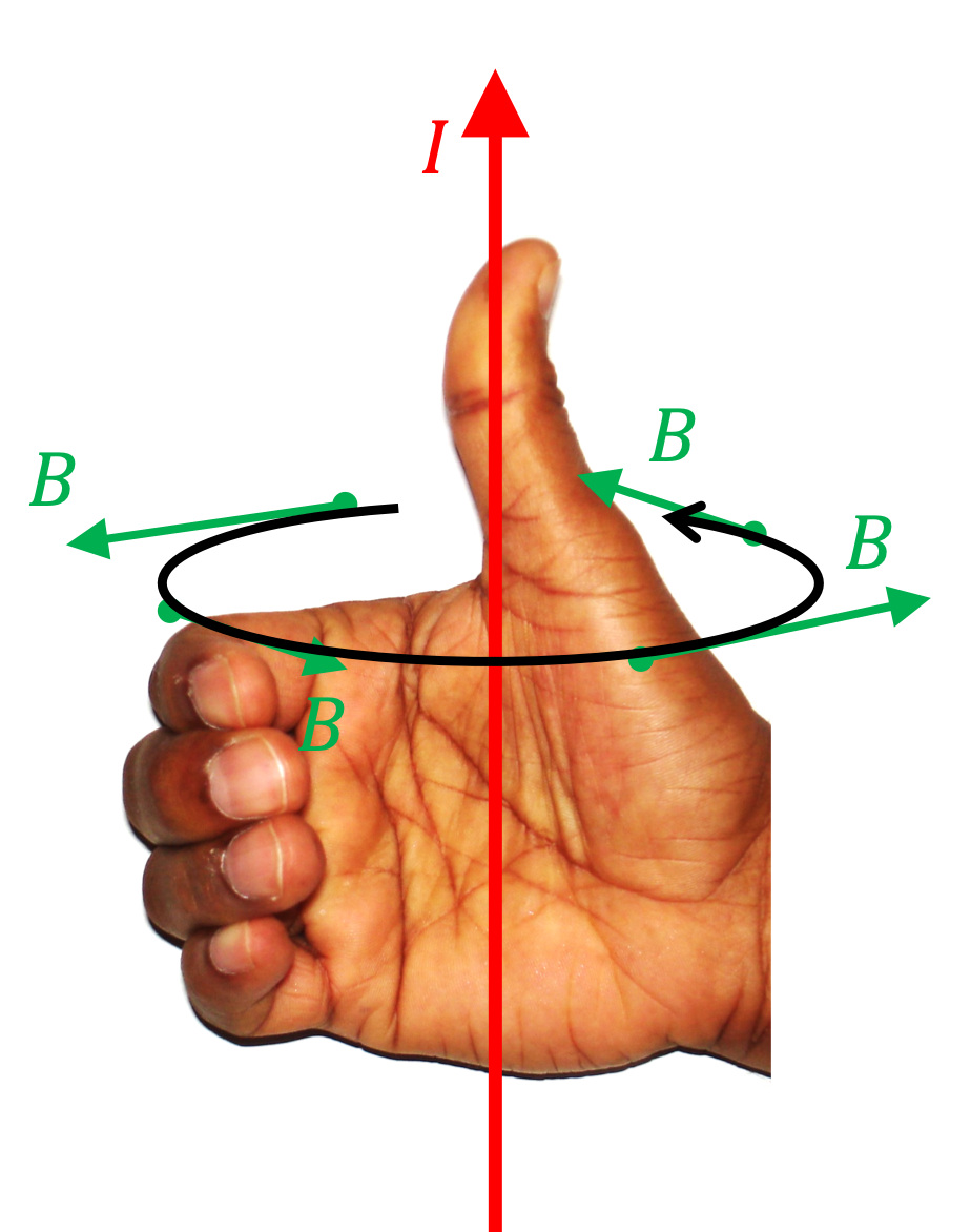
\amp \text{Direction: Use the right-hand-rule of Biot-Savart Law,} \end{align*}

We want to use Ampere's law to find this answer. We will follow the four-step process suggested above.

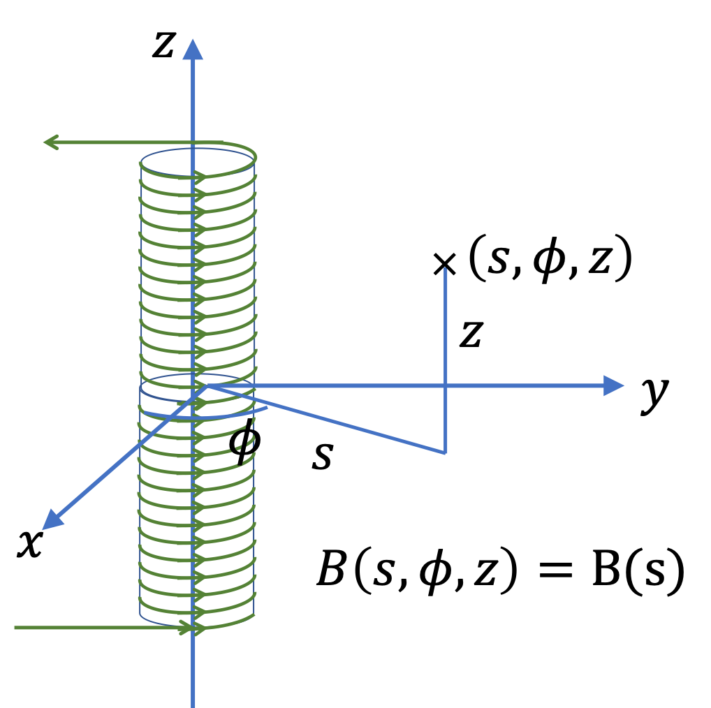
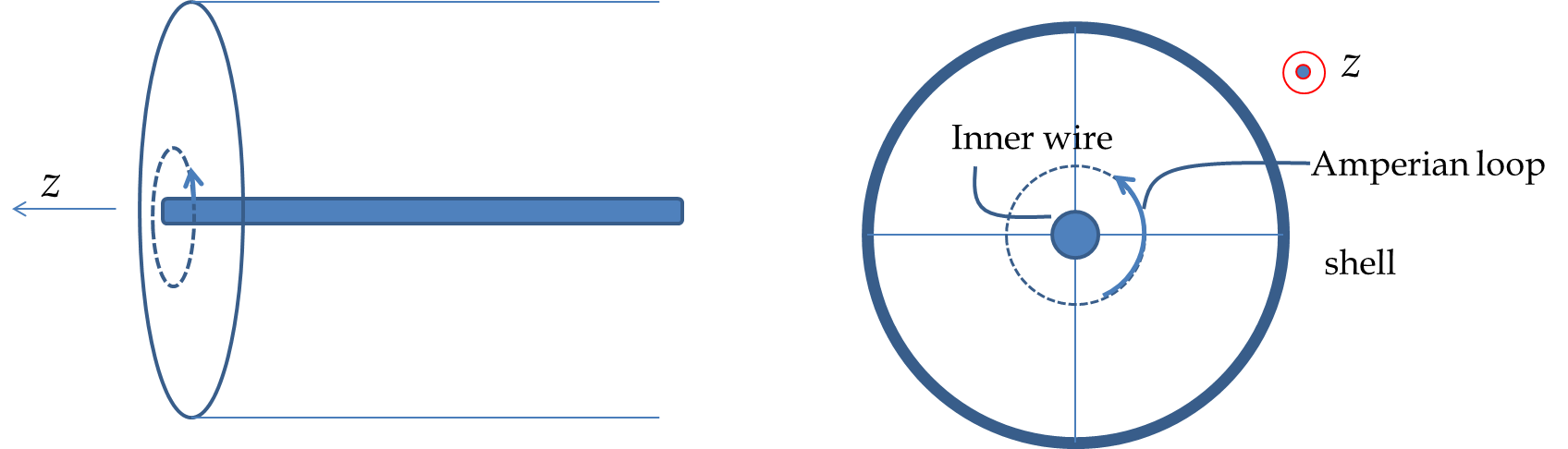
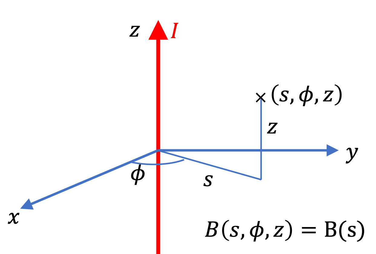
Before we get started, let us look at the current distribution and appropriate coordinate system to use. The current distribution has a cylindrical symmetry. Thereofore, we will use cylindrical coodinate system with coordinates denoted by \((s,\phi, z)\text{.}\) Let current be on the \(z\) axis.

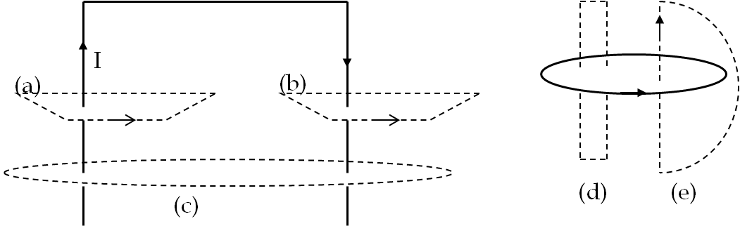
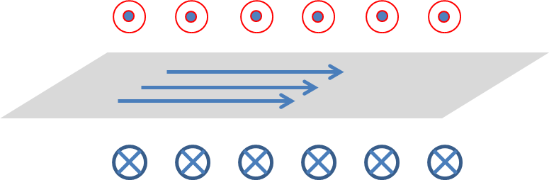
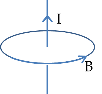
Step 1: What is the direction of magnetic field? Using the Biot-Savart right hand rule, we find that magnetic field will circulate around the wire in circles. At any point it is in the unit vector of cylindrical coordinates, \(\hat u_\phi\) ,direction.

Step 2: What is the functional form of magnitude of the magnetic field? Since current runs on the entire \(z\) axis, nothing can depend on \(z\) coordinate of a point. Also, there is no directional dependence in the current distribution, so, we don't expect any \(\phi\) dependence. Therefore, we conclude that \(B(s,\phi, z) = B(s)\text{,}\) i.e., only \(s\)-dependent. That means magnitude will be same at all points on a circle centered at the \(z\) axis.

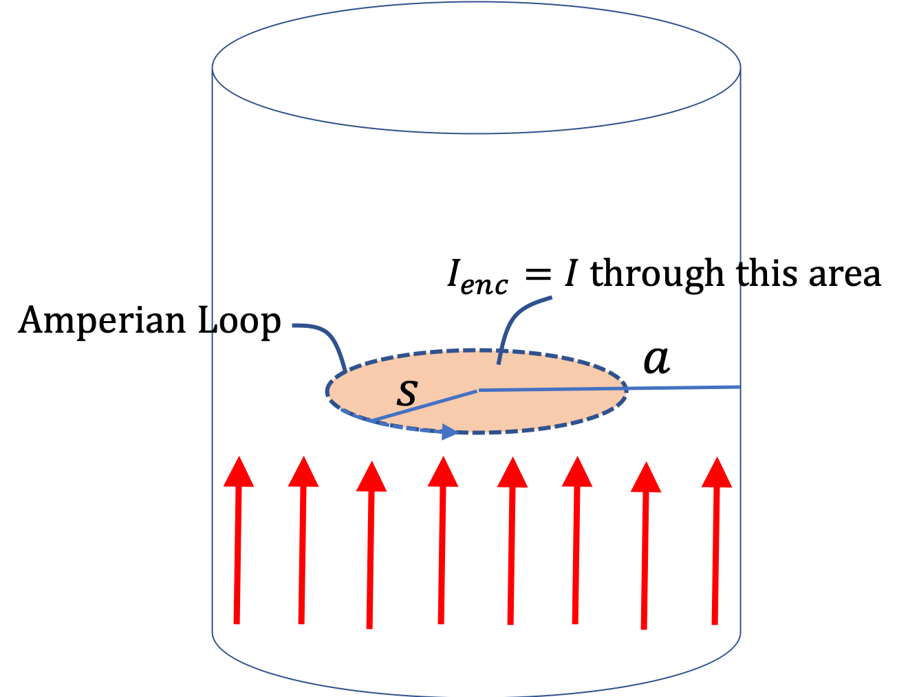
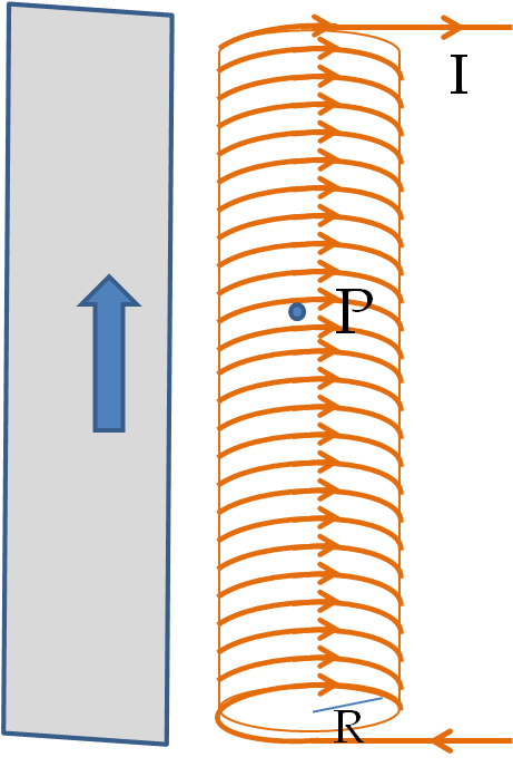
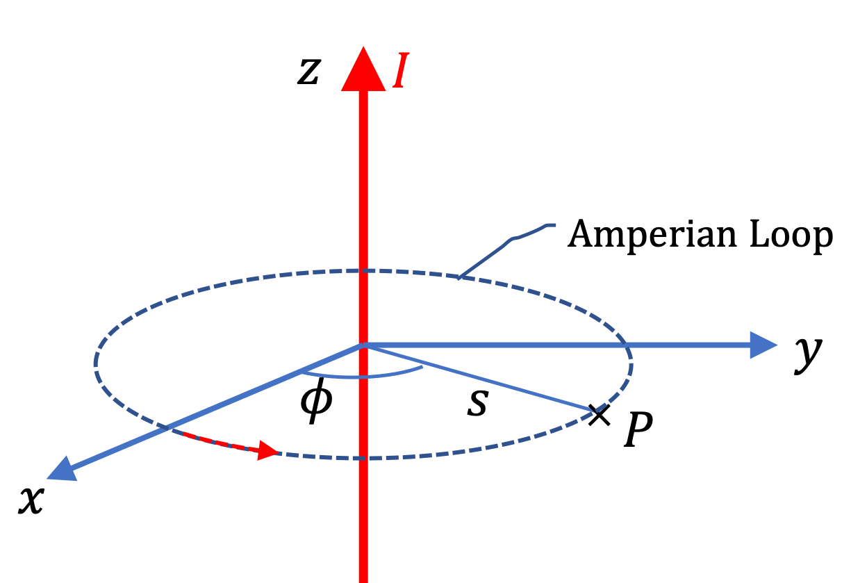
Step 3: Choose Amperian Loop. Let field point P be located at a distance \(s\) from the \(z\) axis. Based on information in steps 1 and 2, if we choose a circle of radius \(s\) with direction \(\hat u_\phi\text{,}\) the magnitude at points of the Amperian loop will be same and the loop direction will be parallel to the field direction.

Step 4: Calculations.

We note that \(B=B_P\) at all points of Amperian loop with direction of loop and field parallel. Therefore, left side of Ampere's law

\begin{equation*} \text{Left side } = 2\pi s B_P. \end{equation*}

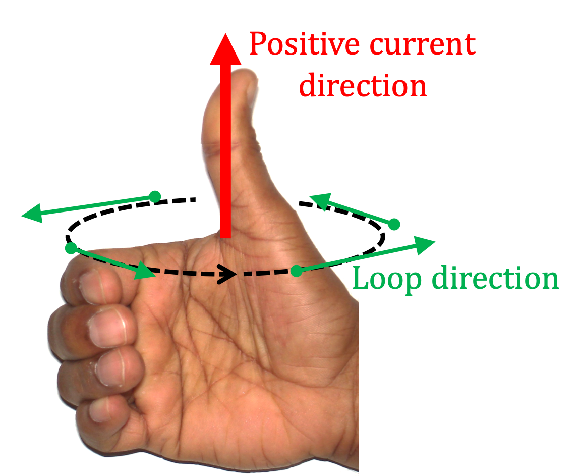
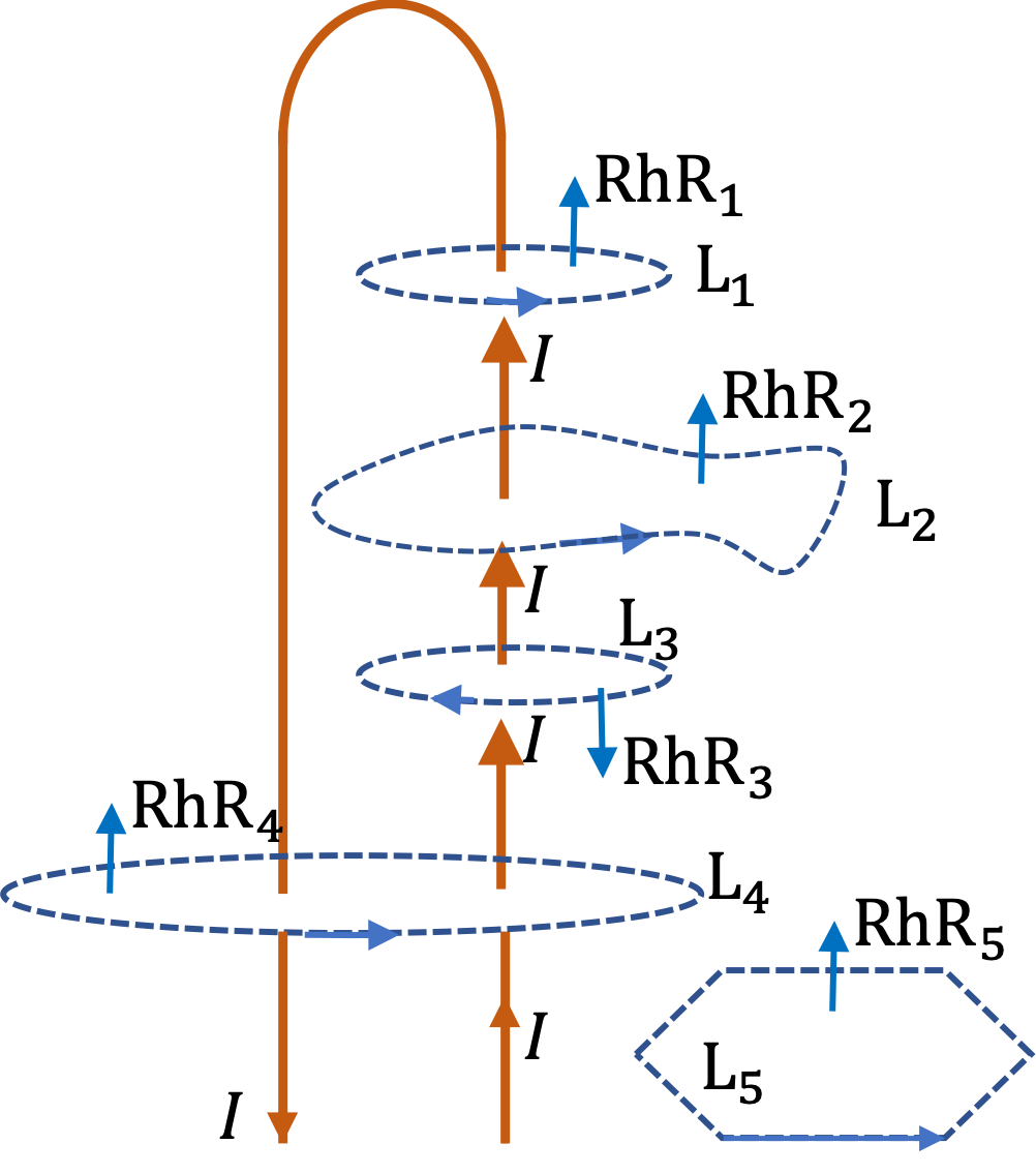
For \(I_\text{enc}\) we notice that entire current passes through the loop in the positive current direction, as seen by applying right-hand rule on the loop direction. Therefore,

\begin{equation*} I_\text{enc} = I. \end{equation*}

Using these in Ampere's law we get

\begin{equation*} 2\pi s B_P = \mu_0, I. \end{equation*}

Therefore, magnitude of magnetic field is

\begin{equation*} B_P = \dfrac{\mu_0}{2\pi}\, \dfrac{I}{s}. \end{equation*}

We have already worked out the direction of the field in step 1 above.

Current \(I \) flows through a thick long wire of radius \(a\text{.}\) Suppose current density is uniformly distributed over the cross-section of the wire. What will be magnetic field at an interior point of the wire?

We will use logic explained in Example 39.4.3. So, if you have not done that problem yet, you need to go back and familiarize yourself of my techniques.

Let \(s\) be the cylindrical radial coordinate for the field point P. Since P if interest is inside \(s \lt a\text{.}\) Our Amperian loop will be a circle of radius \(s\) as for the thin wire. This will give the following for the left side of Ampere's law.

\begin{equation*} \text{Left side } = 2\pi s B_P. \end{equation*}

We find \(I_\text{enc}\) by asking: what the the current that flows the Amperian loop? Note, I am not asking what is the current or what is the current in the wire. Since current density is constant this will just be propoetional to the area. The current through the Amperian loop is

\begin{equation*} I_\text{\enc} = \dfrac{I}{\pi a^2}\times \pi s^2 = I \dfrac{s^2}{a^2}. \end{equation*}

Using this in Ampere's law we get

\begin{equation*} 2\pi s B_P = \mu_0 I \dfrac{s^2}{a^2}. \end{equation*}

Therefore, the magnitude of magnetic field at P is

\begin{equation*} B_P = \dfrac{\mu_0}{2\pi a^2} I\,s. \end{equation*}

Note that current increases with cylindrical radial distance while inside the wire. Outside, the formula will be identical to what we found in Example 39.4.3 since for those points, Amperian loops will include all current in the wire. The direction of the field is obtained in Step 1 by using Biot-Savart right-hand rule.

A good way to produce a known constant magnetic field is by an important device called solenoid. You can make a solenoid by tightly winding a platic-coated wire about a cylinder. Suppose, there are \(n\) turns of the wire per unit length. Suppose, you connect the two ends of the wire to a DC-voltage source and wait till current in the wire has stabilized to a value \(I\text{.}\) Let \(R\) be the radius of each coil. Now, we wish to find magnetic field at a point inside the tube and a point outside the tube.

Suppose solenoid is oriented so that its axis is at the \(z\) axis. If we extend the solenoid to \(z=\pm \infty\text{,}\) we will get one aspect of cylindrical symmetry, making expected magnetic field independent of the coordinate \(z\text{.}\) Another aspect is the direction in the \(xy\) plane. If we wind the coils tightly, each turn will be identical to the next and situation in every direction will be same. With this, \(B\) will also be independent of \(\phi\text{.}\)

Therefore, we come to conclusion that magnitude of magnetic field \(B\) can only be a function of the cylindrical radial coordinate \(s\text{.}\)

\begin{equation*} B(s,\phi, z) = B(s). \end{equation*}

Physically, magnetic field should weaken with increasing radial distance from the solenoid axis. So, we expect

\begin{equation} \lim_{s\rightarrow \infty} B(s) = 0.\label{eq-solenoid-zero-mag-field-at-infinity}\tag{39.4.3} \end{equation}

Using Biot-Savart right-hand rule, the direction inside will be towards positive \(z\) axis and outside it would be towards negative \(z\) axis.

(a) For field point outside the loop, the Amperian loop will be a rectangular shape with two sides parallel to axis at radial distanes \(s>R\) and \(s'>s\text{.}\) Then, left side of Ampere's law gives

\begin{equation*} \text{Left side } = B_P l_\text{ab} + 0 - B(s') l_\text{cd} + 0. \end{equation*}

Here the zeros come from the fact that \(\vec B\) is perpendicular to those sides. The right side of Ampere's law will be zero since no current goes through this Amperian loop.

Therefore, we get the following equation from Ampere's law.

\begin{equation*} B_P l_\text{ab} - B(s') l_\text{cd} = 0. \end{equation*}

Let us take the further side at \(s'\) to \(s'=\infty\text{.}\) That will give

\begin{equation*} B_P l_\text{ab} = B(\infty) l_\text{cd} = 0\times l_\text{cd} = 0. \end{equation*}

Therefore,

\begin{equation*} B_P = 0.\text{ (point P outside)} \end{equation*}

We often write this result as

\begin{equation*} B_\text{out} = 0. \end{equation*}

(b) For field point inside the loop, the Amperian loop will be a rectangular shape with two sides parallel to axis at radial distanes \(s\lt R\) and \(s' \gt R\text{.}\) Then, left side of Ampere's law gives

\begin{equation*} \text{Left side } = B_P l_\text{ab} + 0 - B(s') l_\text{cd} + 0 = B_P l_\text{ab}. \end{equation*}

To obtain the enclosed current, we look at how the wires pierce the Amperian loop area. In each turn, wire carries current \(I\) through the Amperian loop, and all the loops carry current in the same direction. Therefore, current will equal number of turns times \(I\text{.}\)

\begin{equation*} I_\text{enc} = n l_\text{ab}\, I. \end{equation*}

Now, we use Ampere's law,

\begin{equation*} B_P l_\text{ab} = \mu_0 n l_\text{ab}\, I. \end{equation*}

Therefore,

\begin{equation*} B_P = \mu_0 n \, I.\text{ (point P inside)} \end{equation*}

We often write this result as

\begin{equation*} B_\text{in} = \mu_0 n \, I. \end{equation*}

Coaxial cables have a conducting wire at the center and a conducting cylindrical shell surroundng the wire separated by a nonconducting material. Current \(I\) in the center wire and the shell run in opposite directions. What is the magnetic field at a point at a distance \(a\) from the center that is located between the the central wire and the the shell?

Hint

Cylindrical symmetry with only inner wire.

Answer

\(\dfrac{\mu_0}{4\pi}\,\dfrac{I}{a}\text{.}\)

Solution

The Amperian loop will be a circle of radius \(a\) with enclosed current will the current in the wire. The current in the shell does not matter for Ampere's law since it is outside. This problem is same as the problem of a single straight wire. Thus, we can immediately write the answer.

\begin{equation*} B = \dfrac{\mu_0}{2\pi}\,\dfrac{I}{a}. \end{equation*}

The directionn will be obtained by right hand rule and will be either closkwise or counterclockwise around the wire.