Physics Bootcamp

Subsection 55.7.1 Orbital Angular Momentum

A charged particle of charge \(q\) and mass \(m\) with angular momentum \(\vec L\) has a magnetic moment \(\vec \mu\) proportional to the angular momentum.

For an electron, the charge is \(q = -e\text{.}\) Therefore, the magnetic dipole moment of an electron will be

The quantity \(e/2m_e\text{,}\) the proportionality of angular momentum and magnetic dipole moment, is called the gyromagnetic ratio. How can an electron have magnetic property? You may recall from your studies of magnetic field from an electric current loop that a current loop of area \(A\) and current \(I\) can be thought of as a magnetic dipole with the magnetic dipole moment equal to the product of the current and the area of the loop:

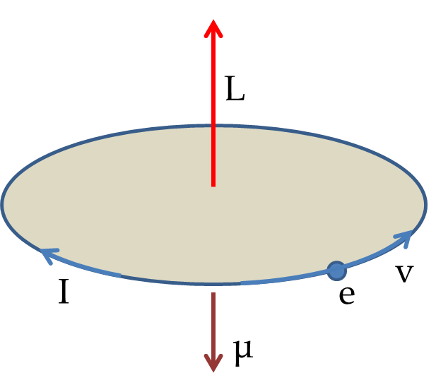
You can model the motion of electron about the nucleus as a motion of uniform speed \(v\) in a circle of radius \(R\) [even if we do not know if this is actually happening or not]. This model allows us easy calculation of angular momentum and think of electron motion as a current. The magnitude of the angular momentum will be

The movement of the charge would give an ``electric current'' \(I\) given by charge divided by the period of the motion in the circle.

Multiplying this with the area of the circle will be equal to the magnitude of the magnetic dipole moment.

Substituting \(vR\) by \(L/m_e\) gives the desired relation between the magnetic dipole moment and the angular momentum given in Eq. (55.7.2).

Since the angular momentum of an electron in an atom is a multiple of \(\hbar\text{,}\) it makes sense to introduce a reference magnetic moment corresponding to \(L = \hbar\text{.}\) This reference magnetic dipole moment is called Bohr magneton and usually denoted by \(\mu_B\text{.}\)

Putting the numerical values we get Bohr magneton to be

Since \(|\vec L|\) and \(L_z\) are quantized, the magnitude of magnetic dipole moment \(|\vec \mu|\) and the \(z\)-component of the magnetic dipole moment \(\mu_z\) will be quantized also. For instance, if \(l=2\text{,}\) then \(|\vec L| = \sqrt{2(2+2} \hbar = \sqrt{6}\hbar\text{,}\) and \(L_z\) can have values \(-2\hbar,\ -\hbar,\ 0,\ +\hbar\text{,}\) and \(+ 2\hbar\text{.}\) The corresponding allowed values of the magnetic dipole moment and its \(z\)-components will be:

Subsection 55.7.2 Normal Zeeman Effect

Since electrons have magnetic dipole moments, they will interact with an external magnetic field. The energy of interaction of a magnetic diople \(\vec \mu\) with an external magnetic field \(\vec B\) is given by

Suppose, the magnetic field is pointed towards the positive \(z\)-axis.

Then, the energy of interaction will be

Therefore, the energy of the states with positive \(\mu_z\) will have lower energy than the states with negative \(\mu_z\text{.}\) It is instructive to write this in terms of the \(m_l\) quantum number of the state.

Thus, the states with negative \(m_l\) will be lower in energy than the states with positive \(m_l\text{.}\) The quantity within parenthesis is the Larmor frequecy of the classical dipole magnetic moment rotating about the external magnetic field and is denoted by \(\omega _L\text{.}\)

The quantity \(\hbar\omega_L\) is called the Zeeman energy. In terms of Zeeman energy the interaction energy of the magnetic dipole of state with magnetic quantum number \(m_l\) is

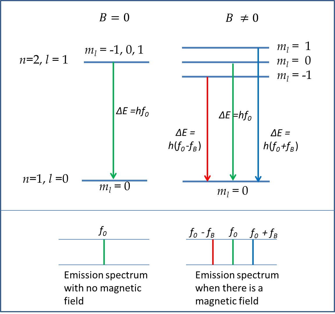
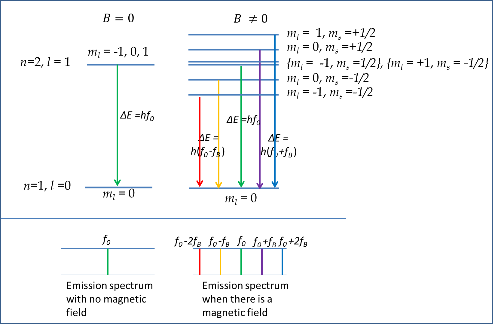
Illustration of Splitting of \(n=2,\ l=1\) States:

Without the magnetic field on, the electron in \(n=2\) state has energy \(E_2\) regardless of the values of \(l\) or \(m_l\text{.}\) When the magnetic field is applied, the energy of the \((l=1, m_l=-1)\) will be lowered by the amount \(1\mu_B B\) with respect to the state with \((l=1, m_l=0)\) and the energy of the state \((l=1, m_l=1)\) will be raised by the amount \(1\mu_B B\) with respect to the state with \((l=1, m_l=0)\text{.}\) We say that the energy of state \(l=1\) is split into three levels as shown in Figure 55.7.2.

This effect can be seen in emisison spectrum of H-atom for the line \(n=2\) to \(n=1\) transition with and without magnetic field on as illustrated in Figure 55.7.2. When magnetic field is on, we see three spectral lines where there is only one line without the magnetic field. The separation in frequency of the line is proportional to the energy difference of the new levels, which is proportional to the applied magnetic field. Thus, as magnetic field is varied, the frequency separation of the lines increases with the magnetic field. The spitting of the spectral lines when magnetic field is applied to the sample is called Zeeman effect, or the normal Zeeman effect. The observation of the Zeeman effect is complicated by the fact that an electron carries an intrinsic angular momentum, called spin, which we will discuss below. The more complicated Zeeman effect that takes into account the effect of spin on the energy levels is called anomalous Zeeman effect.

Subsection 55.7.3 Spin Angular Momentum

Stern-Gerlach Experiment

An atom in \(l=0\) state is expected to have a zero magnetic dipole moment. Therefore, energy of such an atom will not be affected by the presence of a magnetic field. Neither, there will be a magnetic force on an atom in \(l=0\) state. On the other hand, the energy level of an atom in \(l=1\) state is split into 3 levels by a magnetic field. Similarly, the energy of an atom in \(l=2\) state is split into 5 energy levels by a magnetic field. In every case of non-zero \(l\text{,}\) the energy level of the atom is split into odd number of levels - never in an even number of levels - as long as the story of atoms told so far in this chapter is complete.

One can study the effect of magnetic field on the atoms not only in terms of the shifting of energy levels and consequent change in the emission spectrum as illustrated in Figure 55.7.2 but also in terms of the force on atoms in an inhomogeneous field. Let there be a space-dependent (i.e., inhomogeneous) magnetic field \(\vec B(\vec r)\) act on a magnetic dipole \(\vec \mu\text{.}\) Then, there will be a force on the dipole given by

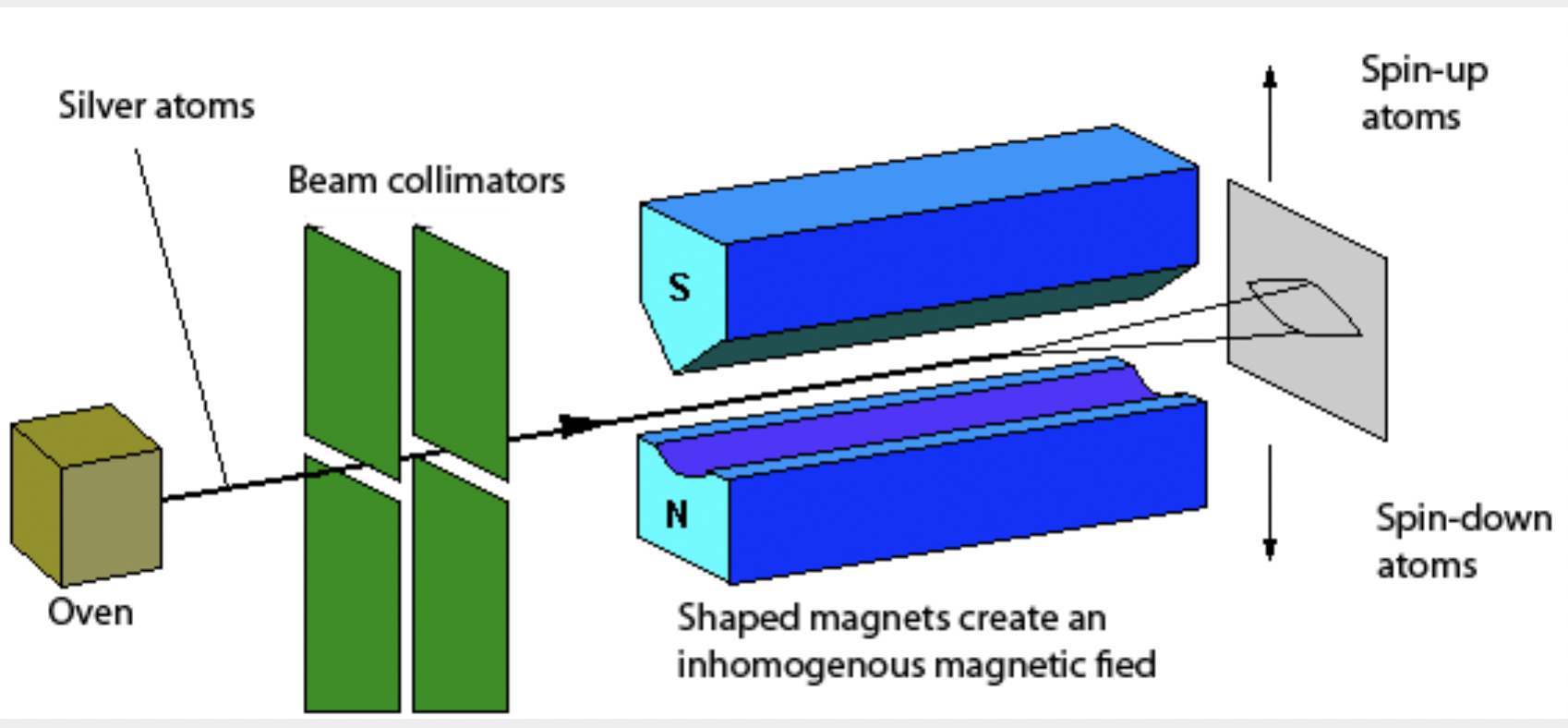
which follows from \(\vec F = -\vec\nabla U\) with \(U = -\vec \mu\cdot \vec B\text{.}\) Atoms with different \(\vec \mu\) will experience different force. For example, if you send atoms in \(l=1\) but different values of \(m_l= -1,\ 0,\ 1\) into a region of inhomogeneous magnetic field, atoms of different \(\mu_z\) will experience different force. Consequently, one beam of atoms would separate into three beams. With \(l=0\) you expect one beam in, one beam out, with \(l=2\text{,}\) you expect one beam in and 5 beams out, etc.

In 1921 Walter Gerlach conducted an experiment in collaboration with Otto Stern on silver atoms in \(l=0\) state. A schematics of their apparatus is shown in Figure 55.7.3. A silver atom beam from an oven was sent through the space between poles of a magnet, where magnetic field was inhomogeneous, separated into two beams! This was a complete surprise since, if \(l\) were anything nonzero, there would be an odd number of beams out and if \(l=0\) there should be a single beam out. Their result could not be explained on the basis of the connection of \(l\) values to the magnetic dipole moment.

The explanation came from Samuel Goudsmit and George Uhlenbeck, who were at the time graduate students at the University of Leiden, Germany. They proposed that the origin of magnetic dipole moment was the “spinning” of electrons. With this proposal they were successful in explaining a number of anomalies with the Zeeman effect due to the presence of additional source of magnetic dipole moment than could be accounted for by the orbital angular momentum \(l\text{.}\) Now, we know that the additional magnetic moment is not due to a physical spinning of the electron but rather an intrinsic angular momentum, which does not have a classical analog. The additional angular momentum is called spin, which is an intrinsic property of elementary particles.

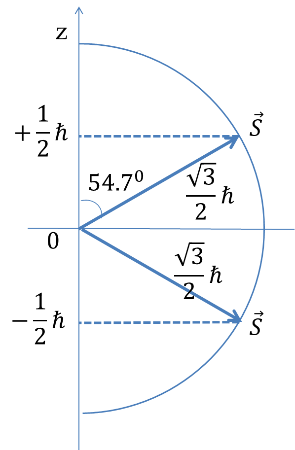
Similar to the orbital angular momentum, the spin angular momentum \(\vec S\) is also quantized so that its magnitude \(|\vec S|\) is specified by particular quanta. For electrons, the magnitude of spin is \(\frac{\sqrt{3}}{2}\hbar\text{.}\) Spin angular momentum also exhibits space quantization similar to the way orbital angular momentum is space-quantized so that the components of the spin angular momentum vector in any direction, say the \(z\)-axis, \(S_z\) take discrete values. In the case of electron, the space quantization leads to the electron having spin angular momentum component equal to either \(+\frac{1}{2}\hbar\) or \(-\frac{1}{2}\hbar\) in any direction as shown in Figure 55.7.4. We usually take the direction of reference to be the positive \(z\)-axis.

The quantized components \(+\frac{1}{2}\hbar\) and \(-\frac{1}{2}\hbar\) are called up spin and down spin respectively. They are often denoted by arrow pointed up and down respectively.

For a general spin situation, let us denote the spin quantum number by letter \(s\) and the quantum number for the components of the spin in a direction by \(m_s\text{.}\) The magnitude and projections of the angular momentum vector follow similar rules as was the case with the orbital angular momentum.

However, the similarities between spin and orbital angular momenta are quite deceptive. While the orbital angular momentum can be understood from the motion of the electron about the nucleus, there is no easy way to understand the spin. Additionally, the magnetic dipole moment \(\vec \mu_s\) associated with the spin angular momentum is actually twice as strong as the magnetic dipole moment associated with the orbital angular momentum. We introduce a multiplicative factor \(g\text{,}\) called the Landé g factor, to the gyromagnetic ratio to write the ratio of magnetic moment and spin angular momentum.

The Land\'e g factor has a value of approximately 2 for an electron. The \(g\) factor was quite a mystery in the early days of quantum mechanics until the British physicist/mathematician Llewellyn Thomas performed a calculation using relativity and convinced the reality of the quantum number spin. The total magnetic moment of an electron in hydrogen atom would come from both the orbital and spin angular momenta.

Anomalous Zeeman Effect

We have discussed above that a magnetic dipole in a magnetic field has an interaction energy given by

We found above that when \(l\ne 0\text{,}\) the energy level of a hydrogen atom is split into additional levels with energy dependent upon the projection of the magnetic dipole vector in the direction of the magnetic field. Now, there is another source of magnetic moment - due to the spin of the electron. That causes further splitting of the levels. For concreteness, let us consider a magnetic field pointed in the positive \(z\)-direction.

This will give the following interaction energy

The allowed values of \(L_z\) are \(L_z = m_l \hbar\) with \(m_l\) ranging from \(-l\) to \(+l\) in integer steps and the allowed values of \(S_z\) are \(S_z = m_s\hbar\) with \(m_s = -1/2\) and \(m_s = +1/2\text{.}\) Let us rewrite Eq. (55.7.19) in terms of \(m_l\) and \(m_s\text{,}\) and write the constants as Bohr magneton.

Let us examine the energy of \((n=2, l=1)\) level of H-atom with and without magnetic field. The energy of this level in the absence of magnetic field depends only on the principal quantum number \(n\text{.}\) We will denote the energy of this level by \(E_2\) as before. Now, when magnetic field is on, the energy level will split into five energy levels due to various \(m_l\) and \(m_s\) values. We will label the new energy levels with \(n,l, m_l, m_s\) values to be complete. Using \(g=2\) the energy levels are:

Figure 55.7.5 shows the energy diagram of the new energy levels and emission spectrum from emission from \(n=2, l=1\) levels to \(n=1\) level. There are six possible combinations of the three \(m_l\) values and two \(m_s\) values. Two of the these combinations, namely \((m_l=-1, m_s = +\frac{1}{2})\) and \((m_l=+1, m_s = -\frac{1}{2})\) have the same energy. Therefore, we get a total of five distinct energy levels when \(B\ne 0\text{.}\)

Subsection 55.7.4 The Spin-Orbit Interaction

We have seen above that magnetic dipole \(\vec \mu\) due to orbital and spin angular momenta interact with the external magnetic field \(\vec B_{ext}\text{.}\) The interaction energy is given by

This interaction energy causes the energy levels to shift up or down depending on \(m_l\) and \(m_s\) and the magnetic field \(B_{ext}\text{.}\) Therefore, it would appear that you need an external field to split the energy levels based on magnetic effect. However, this is not true as the electron itself produces a magnetic field due to the orbital motion. The state with angular momentum quantum number \(l\ne 0\) an be though of an electron moving in an orbit, which constitutes a current, which produces a magnetic field, \(\vec B_l\text{.}\)

The magnetic moment \(\vec \mu_s\) due to spin angular momentum then interacts with this magnetic field.

This would give rise to a magnetic energy,

A quantum mechanical calculation shows that

where

where \(V_c\) is the effective potential of the electron, which takes into account the interaction with the nucleus and other electrons. We will not go into the details of \(c(r)\text{,}\) but treat Eq. (55.7.21) as stating that if \(\vec S\) is in the same direction as \(\vec L\text{,}\) the energy will be shifted up and if \(\vec S\) is in the opposite direction to \(\vec L\text{,}\) the energy will be shifted down.

As an example, consider the case of a sodium atom. The ground state of sodium atom has a lone electron in the outer shell,

The ten electrons of the Ne core can be thought to shield out 10 of the 11 protons of the nucleus, leaving Na atom as an outsized hydrogen atom. The outermost electron in \(3s^1\) can be excited to higher states and when they de-excite, they would emit photons. Even though, Na appears formally to be like H atom, the energy of states depend on both \(n\) and \(l\text{,}\) not just \(l\text{.}\) Thus, in Na the \(3s\) and \(3p\) states are at different energy. In general, the energy goes as the square of \((n+l)\) rather than just the square of \(n^2\text{.}\)

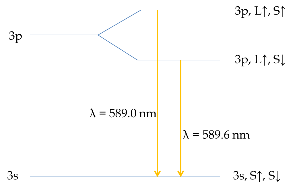
With the lifting of the degeneracy of \(3s\) and \(3p\) states, the nearest level to excite from the \(3s\) is the \(3p\) state. Now, \(3p\) state has \(l=1\text{.}\) The energy of the \(3p\) state will depend on whether the angular momentum vector \(\vec L\) is in the same direction as the spin \(\vec S\text{.}\) Let us use the notation of up-spin and down-spin for direction specification. We will say, that up spin is the direction in which both \(\vec L\) and \(\vec S\) are in the same direction, then down-spin will be the direction in which \(\vec S\) will be in the opposite direction of \(\vec L\text{.}\) This would mean that \(\uparrow\) spin will have higher energy than the \(\downarrow\) spin due to the spin-orbit coupling.

Thus, there would be two energy levels within the \(3p\) state, one \(3p_{\uparrow}\) and the other \(3p_{\downarrow}\text{.}\) The transitions from these two states will differ in energy as illustrated in Figure 55.7.6. This is exactly what we see in the spectroscopy of sodium atom. The \(3p\) to \(3s\) transition gives two closely-spaced lines, called the sodium doublet, at wavelengths \(\lambda = 589.6\) nm and \(\lambda = 589.0\) nm. The splitting of \(3p\) levels, one for spin up and the other for spin down, is called fine structure.