Velocity from Acceleration

Section 4.6 Velocity from Acceleration

Acceleration and velocity have the same mathematical relation as velocity and position do.

\begin{equation} \vec a = \frac{d\vec v}{dt }\ \ \leftrightarrow \ \ \vec v = \frac{d\vec r}{dt }.\tag{4.40} \end{equation}

Therefore, as in the last section Section 4.5, formally, change in velocity vector will be related to the integration of acceleration over time.

\begin{equation} \vec v_f - \vec v_i = \int_{t_i}^{t_f} \vec a(t) dt.\tag{4.41} \end{equation}

This formal relation can be given more calculational interpretation when we look at the components of this equation.

\begin{align} \amp v_{f,x} - v_{i,x} = \int_{t_i}^{t_f} a_x(t) dt, \tag{4.42}\\ \amp v_{f,y} - v_{i,y} = \int_{t_i}^{t_f} a_y(t) dt, \tag{4.43}\\ \amp v_{f,z} - v_{i,z} = \int_{t_i}^{t_f} a_z(t) dt. \tag{4.44} \end{align}

The right side of these equations for components, can be computed from plots of corresponding acceleration component versus time by using the "area-under-plot" and "negative-area-over-plot" interpretation of an integral.

Example 4.55. Area under the Acceleration Plot.

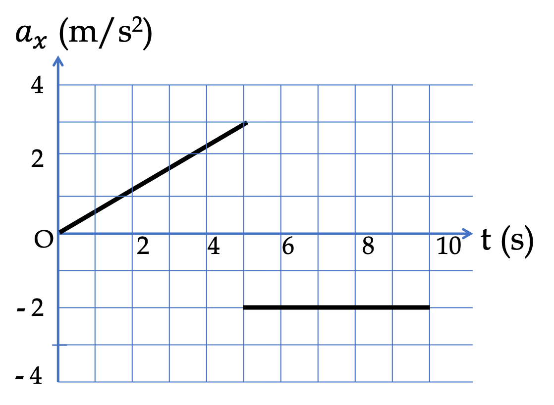
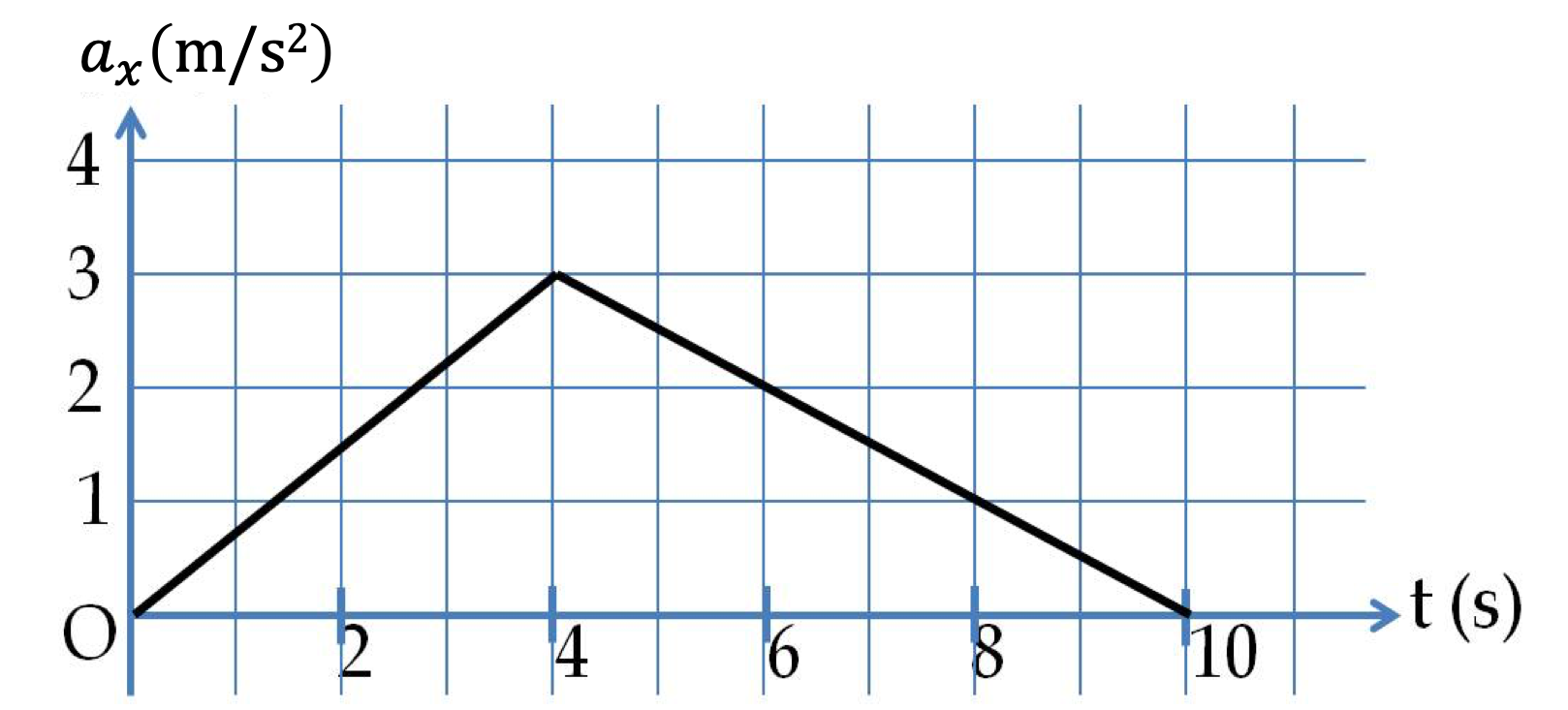
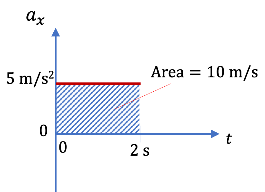
We can understand Eq. (4.42) in a plot of \(a_x\) vs \(t\) as well. Since \(a_x\) is constant, the product \(a_x \Delta t\) is just the area under the plot of \(a_x\) vs \(t\text{.}\) This gives us following general rule, which also applies to varying \(a_x\text{.}\)

\begin{align*} \Delta v_x \amp = \text{ Area under }a_x\text{ vs } t,\\ \amp = 5\text{ m/s}^2 \times 2\text{ s} = 10 \text{ m/s}. \end{align*}

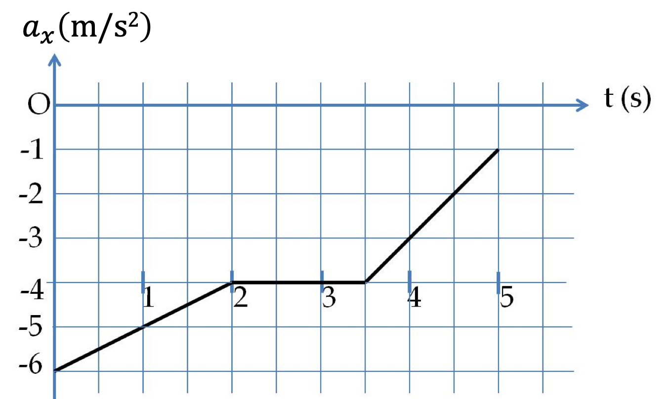
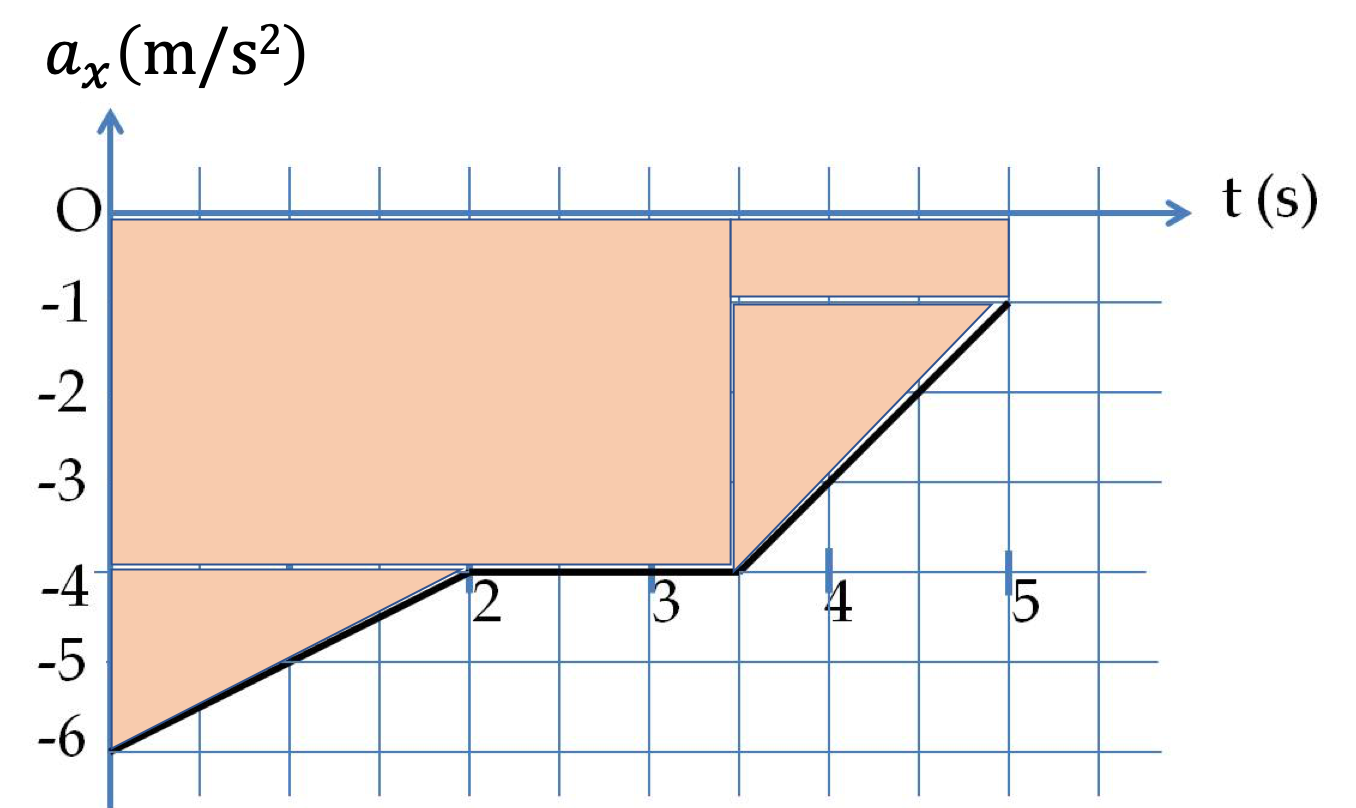
If \(a_x\) is negative, then this would be area above the plot since \(a_x=0\) line would be above the plot. In this case area will be negative.

The procedure clearly extends to \(y \) and \(z \) components as well. Once we know the change along different directions, we can combine the components to obtain the magnitude and direction of \(\Delta \vec v\text{,}\) as usual for vector quantities.

Example 4.56. Velocity from Acceleration - Areas Under Curve.

Figure 4.57 below shows acceleration component \(a_x \) of a ball at different times. The \(x\) component of the velocity of the ball at \(t = 0 \) was \(v_x = 3 \text{ m/s}\text{.}\) Find its \(v_x \) at the following instants (a) \(t = 5\text{ sec}\text{,}\) and (b) \(t = 10\text{ sec}\text{.}\)

Answer.

(a) \(10.5\text{ m/s}\text{,}\) (b) \(0.5 \text{ m/s}\text{.}\)

Solution 1. a

We will find the change in \(v_x \) during \(t=0\) to \(t=5\text{ sec}\text{.}\) Then we will get \(v_x \) at \(t=5\text{ sec}\) by adding this change to the \(v_x \) at \(t=0\text{.}\)

\begin{equation*} v_x(\text{at } t=5\text{ sec}) = v_x(\text{at } t=0) + \Delta v_x, \end{equation*}

where

\begin{equation*} \Delta v_x = \text{Area under the curve of }a_x \text{ between }t=0\text{ and }t=5. \end{equation*}

From the plot we find this to give

\begin{equation*} \Delta v_x = \dfrac{1}{2}\times 5\text{ s} \times 3 \text{ m/s}^2 = 7.5\text{ m/s}. \end{equation*}

Therefore,

\begin{equation*} v_x(\text{at } t=5\text{ sec}) = 3\text{ m/s} + 7.5\text{ m/s} = 10.5\text{ m/s}. \end{equation*}

Solution 2. b

We can similarly add to this the area between \(t=5\text{ sec}\) and \(t=10\text{ s}\) to obtain \(v_x\) at \(10\text{ s}\text{.}\) Now the \(\Delta v_x \) is

\begin{equation*} \Delta v_x = 5\text{ s}\times (-2\text{ m/s}^2) = -10\text{ m/s}. \end{equation*}

Therefore, \(v_x \) at \(t=10\text{ s}\) is

\begin{equation*} v_x(\text{at } t=10\text{ s}) = 10.5\text{ m/s} + (-10\text{ m/s}) = 0.5 \text{ m/s}. \end{equation*}

Exercises Exercises

1. Velocity of a Box from Area Under Curve Method Applied to Varying Acceleration.

A box slides on a floor in a straight path such that the magnitude of the acceleration is not constant in time. The data is collected with respect to a Cartesian axis system in which only the \(a_x\) is non-zero. The \(x\)-component of the acceleration is shown in Figure 4.58. As the figure shows, the direction of the acceleration is always pointed towards positive \(x\)-axis, but the magnitude varies with time.

(a) Find the velocity of the box at \(t = 4\) sec if it starts out at rest at \(t = 0\text{.}\)

(b) Find the velocity of the box at \(t = 10\) sec.

Hint.

Area under the curve will give \(\Delta v_x\text{.}\)

Answer.

(a) \(6\text{ m/s}\text{,}\) (b) \(15\text{ m/s}\text{.}\)

Solution 1. a

We work with the duration \(t = 0\) to \(t = 4\text{ sec}\text{.}\) The area under the curve is just area of a triangle of base \(4\text{ sec}\) and height \(3\text{ m/s}^2\text{.}\) Therefore,

\begin{equation*} v_f = v_i + \Delta v = 0 + \dfrac{1}{2}\times 4\text{ s}\times 3\text{ m/s}^2 = 6\text{ m/s}. \end{equation*}

Solution 2. b

We work with the duration \(t = 0\) to \(t = 10\text{ sec}\text{.}\) The area under the curve is just area of a triangle of base \(10\text{ sec}\) and height \(3\text{ m/s}^2\text{.}\) Therefore,

\begin{equation*} v_f = v_i + \Delta v = 0 + \dfrac{1}{2}\times 10\text{ s}\times 3\text{ m/s}^2 = 15\text{ m/s}. \end{equation*}

2. Velocity of a Hockey Puck from Area Under Curve Method Applied to Varying Acceleration.

A hockey puck is shot on a surface that has different roughness at different places. As a result its acceleration varies from place to place. By placing the \(x\)-axis on the line of motion of the puck, we cast the acceleration vector in terms of its \(x\)-component which can be plotted with time. Note the acceleration vector cannot be plotted, since they are not ordinary functions; only the components can be plotted. The resulting \(x\)-component of the acceleration is shown Figure 4.59. The \(y\) and \(z\)-components of the acceleration are zero. The puck has a velocity at \(t = 5\) sec of \(2\) m/s towards the positive \(x\) axis. Find the initial velocity of the puck at \(t = 0\text{.}\)

Hint.

Area under the curve will give \(\Delta v_x\text{.}\)

Answer.

\(21.75\text{ m/s}\text{.}\)

Solution.

The areas we need are shaded in Figure 4.60. The area will be negative here.

I found the area to be

\begin{align*} \Delta v \amp = -4\times 3.5 + (-1 )\times 1.5+ \dfrac{(-6+4) \times 2}{2} + \dfrac{(-4+1)\times 1.5}{2} \\ \amp = -19.75\text{ m/s}. \end{align*}

Therefore,

\begin{equation*} v_f - v_i = \Delta v, \end{equation*}

gives

\begin{equation*} v_i = v_f - \Delta v = 2\text{ m/s} - ( -19.75\text{ m/s}) = 21.75\text{ m/s}. \end{equation*}

Checkpoint 4.61. Velocity of an Elevator from its Acceleration.

An elevator is going up with an acceleration given by \(\vec a = (10.0\, e^{-{2t}})\,\hat u_y\, \text{m/s}^2\text{,}\) where \(t\) is in seconds. If the elevator started from rest, what will be its speed at \(t=3.0\text{ s}\text{.}\)

Answer.

\(5\left(1 - e^{-6} \right)\) m/s.

Solution.

Here, only the \(y\) component is non-zero. By integrating \(a_y\) from \(t=0\) to \(t=3\text{,}\) we will get our answer.

\begin{equation*} v_y(3) - v_y(0) = \int_0^3 a_x dt = \left. 10.0\frac{e^{-2t}}{-2}\right|_{0}^{3} = 5.0 - 5.0 e^{-6}. \end{equation*}

Since the elevator started from rest, we have \(v_y(0)=0\text{.}\) Hence,

\begin{equation*} \vec v = \left( 5.0 - 5.0 e^{-6} \right)\,\hat u_y\,\text{m/s}. \end{equation*}

Therefore, speed at that instant is \(5\left(1 - e^{-6} \right)\text{.}\)

Prev Top Next