Method of Images

Section 32.10 Method of Images

Electric potential of a charge near a metal is quite complicated. Method of images is a special technique that can simplify the calculation. It is based on making sure that the potential function produce potential at all surface points of the metal. We will see this im practice below for a potential of a charge near a flat metal surface.

Figure 32.42(a) shows charge \(+q\) in front of a grounded conductor plate, meaning, electric potential, \(\phi=0\) at surface points of the metal. Let the conducting plane be the \(xy\) plane and the point charge \(+q\) be on the \(z\) axis. We look for a problem that has charge \(+q\) at \(z = h\) and some other charge or charges arranged in such a way that the potential is zero for all point in the z=0 plane.

Figure 32.42. Method of images. (a) A point charge in front of a grounded infinite planar conductor. (b) Two point charges which have a zero potential surface that falls in the same place as the planar conductor’s surface. The negative charge in (b) is called the image charge. Figure (b) without the plate is equivalent to problem in Fig. (a) since they both agree at points above the plate. They disagree at points below the plate.

As shown in Figure 32.42(b), there is a problem indeed that has the desired characteristics: two charges, \(+q\) at \(z = h\) and \(-q\) at \(z = -h\text{.}\) We replace the original problem of one charge in front of a \(V=0\) conducting plane with a problem of two charges \(+q\) and \(-q\) separated by a distance \(2h\) and no conducting plane as displayed in Figure 32.42(b). The electric potential of the problem in Figure 32.42(b) for \(z\ge 0\) is identical to the electric potential of the problem in Figure 32.42(a).

The potential at point P of the two charge system will be same as the potential for one charge and a \(V=0\) infinite plane for \(z\ge 0\) in order to coincide with the boundary condition.

\begin{equation*} \phi_P = \frac{q}{4\pi\epsilon_0}\left[\frac{1}{\sqrt{x^2+y^2+(z-h)^2}} - \frac{1}{\sqrt{x^2+y^2+(z+h)^2}}\right]. \end{equation*}

In Figure 32.43, we show the equipotential lines and the electric field lines in the \(yz\) plane of Figure 32.42. We see that the field lines bend and land perpendicular to the conducting plate where negative charges on the conducting plate is induced.

Figure 32.43. Equipotential and electric field lines for a point charge near a conducting plate.

Subsection 32.10.1 (Calculus) Electric Field for a Charge Near a Grounded Cunductor

From the electric potential for a point charge in front of a plane conductor found above we can determine the electric field by \(\vec E = \vec{\nabla}\phi\text{.}\) The components of the electric field are

\begin{align*} E_x \amp = - \frac{\partial \phi_P}{\partial x}\\ E_y \amp = - \frac{\partial \phi_P}{\partial y}\\ E_z \amp = - \frac{\partial \phi_P}{\partial z} \end{align*}

These components are not very instructive. We do not need to find all three components to get more information about the induced charges on the plates.

Subsection 32.10.2 (Calculus) Distribution of Induced Charges on Metal Plate near a Point Charge

Near the plate, electric field is equal constant with magnitude equal to \(\sigma/\epsilon_0\) and perpendicular to the plates. Therefore, the distribution of negative charges on the plate can be determined from the difference of the normal component of the electric field across the surface.

\begin{align*} \amp E_{z}|_{z>0} - E_z|_{z \lt 0} = \frac{\sigma_\text{ind}(x,y,0)}{\epsilon_0} \end{align*}

where \(\sigma_\text{ind}(x,y,0)\) is the induced charge density distribution on the plate. Using the \(z\) component of the electric field, we find the following for the surface charge density on the plate.

\begin{equation*} \sigma_\text{ind}(x,y,z) = \frac{-qh/2\pi}{\left(x^2+y^2+h^2 \right)^{3/2}} \end{equation*}

The total induced negative charge can be obtained by integrating ind over the plate, which goes to infinity. It is best to do this in the polar coordinates, \((s,\phi,z)\text{.}\) The induced charge on the plate is function of only the radial coordinate \(s\text{,}\) which is integrated of the surface area of \(xy\) plane to yield that the induced charge is equal to the negative of the point charge of the point charge in front of the grounded plane.

\begin{equation*} \sigma_\text{ind}(s) = \frac{-qh/2\pi}{\left(s^2+h^2 \right)^{3/2}} \end{equation*}

We can integrate the surface charge density over the plane and obtain the net charge induced in the plane.

\begin{equation*} q_\text{ind} = \int\sigma_\text{ind} 2\pi sds = -q \end{equation*}

Exercises 32.10.3 Exercises

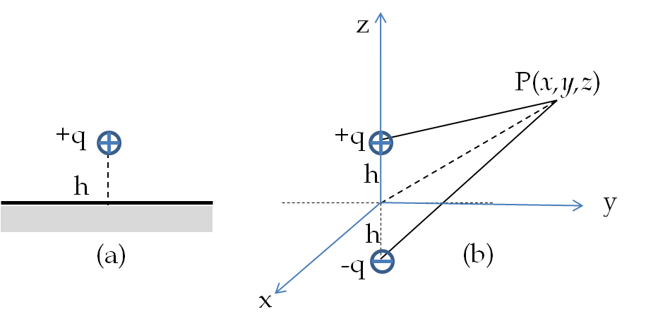
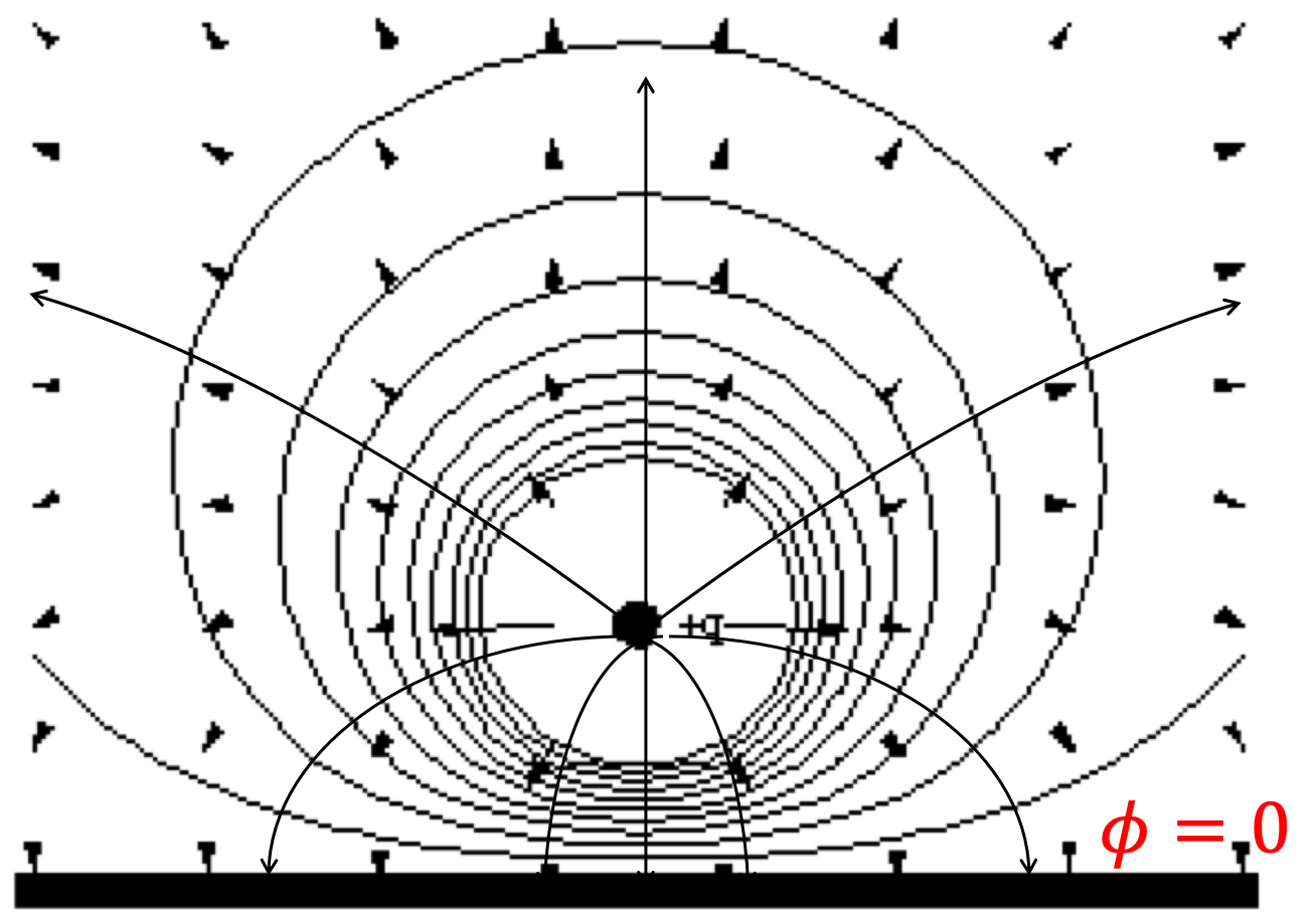
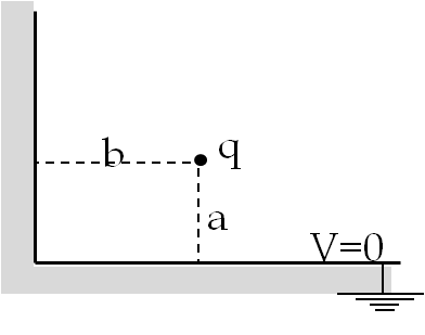
1. Potential of A Charge Near Two Rectangular Plates by Method of Images.

A point charge \(+q\) is placed near a large grounded \((V=0)\) uncharged conductor which is bent at right-angle in the middle. The distance of \(+q\) from the two sides are \(a\) and \(b\text{.}\) Find the force of attraction on \(+q\) by the uncharged conductor.

Solution.

The image charges 1, 2, and 3 are shown in the figure. The net potential of the image charges on the \(x\)- and \(y\)-axes is zero as required in the problem. The force on the real charge \(q\) by the induced charges in the grounded plates can be computed by the force on the real charge by the image charges. The three forces on \(q\) are shown in the following figure.

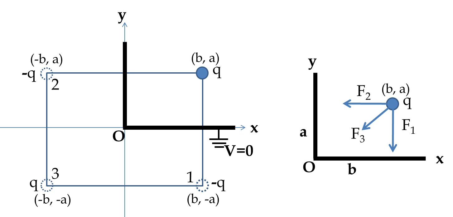
The forces by the image charges have the following magnitudes.

\begin{align*} \amp F_1 = \dfrac{1}{4\pi\epsilon_0}\: \dfrac{q^2}{4a^2},\\ \amp F_2 = \dfrac{1}{4\pi\epsilon_0}\: \dfrac{q^2}{4b^2},\\ \amp F_3 = \dfrac{1}{4\pi\epsilon_0}\: \dfrac{q^2}{4(a^2+b^2)}. \end{align*}

Now, we need to add these forces vectorially. The \(x\) and \(y\) components of these forces are

\begin{align*} \amp F_{1x} = 0,\ \ F_{1y} = - F_1,\\ \amp F_{2x} = -F_2,\ \ F_{2y} = 0,\\ \amp F_{3x} =- F_3 \dfrac{b}{\sqrt{a^2+b^2}},\ \ F_{3y} =- F_3 \dfrac{a}{\sqrt{a^2+b^2}}. \end{align*}

Therefore, the net force on the real charge will have the following \(x\) and \(y\) components.

\begin{align*} \amp F_{x} = -F_2 - F_3 \dfrac{b}{\sqrt{a^2+b^2}},\\ \amp F_y = -F_1- F_3 \dfrac{a}{\sqrt{a^2+b^2}}. \end{align*}

2. Work Required for Bringing a Charge from Far to Near a Grounded Metal Plate.

A point charge is brought from infinity to a distance \(h\) from a grounded plane conductor. Find the amount of work done.

Solution.

Let the grounded plane be the \(x\)-plane and the real charge is brought on the \(z\)-axis from \(z=\infty\) to \(z=h\text{.}\) Note that the image moves as we move the real charge. Consider moving the real charge from a coordinate \(z\) to \(z-dz\text{.}\) The work by the external agent, which would apply the force in thh positive \(z\) direction to balance the electric force from the negatively charged image charge will be

\begin{equation*} dW = \dfrac{1}{4\pi\epsilon_0}\: \dfrac{q^2}{(2z)^2}\: dz. \end{equation*}

Therefore, the net work done over the path from \(z=\infty\) to \(z=h\) will be

\begin{equation*} W = \dfrac{1}{4\pi\epsilon_0}\: \int_{\infty}^{h}\dfrac{q^2}{(2z)^2}\: dz = - \dfrac{1}{4\pi\epsilon_0}\:\dfrac{q^2}{4h}. \end{equation*}

Prev Top Next