Velocity and Speed

Section 2.4 Velocity and Speed

Subsection 2.4.1 Average Speed

Perhaps the crudest measure of how fast something is moving comes from looking at the distance it has covered in a given time. The ratio of the distance convered, \(d \text{,}\) and the time taken, \(t \text{,}\) is called average speed. We will denote average speed by the symbol \(v_{\text{s,av}}\text{,}\) and if there is no confusion in the context, then by simply \(v\text{.}\)

\begin{equation} v_{\text{s,av}} = \dfrac{d}{t}.\tag{2.2} \end{equation}

Suppose you drive a car for a distance of \(4000\text{ km} \) in \(50\text{ hr}\text{.}\) Then your average speed will be

\begin{equation*} v_{\text{s,av}} = \dfrac{4000\text{ km}}{50\text{ hr}} = 80\text{ km/hr}. \end{equation*}

Note that when we are speaking about average speed, we are not concerned with the direction changes during the motion or the overall direction of motion. We are also not refering the varying value of speed along the way. We are concerned with just the length of the path driven and the total time taken on that path.

Example 2.16. Constant Speed Warmup.

You drive your car from New York City to Los Algeles in 50 h at an average speed of 96 km/h. What is the total distance you have traveled?

Answer.

\(4,800 \text{ km}\) .

Solution.

From the definition of average speed, \(v = d/t \text{,}\) we get

\begin{equation*} d = v t = 96 \text{ km/h } \times 50 \text{ h } = 4,800 \text{ km}. \end{equation*}

Subsection 2.4.2 Average Velocity

Another measure of motion has to with the rate of overall movement from the intitial instant to the final instant. Here, we do not care about all the places you visited during the interval, but just where you were at the beginning and where you ended up at the end, i.e., we care about displacement during the interval and not the distance covered. Average velocity is obtained by dividing the displacment by the interval.

If the motion is on the \(x \) axis, we will denote the average velocity by the symbol \(v_{\text{av},x}\text{,}\) which will be the ratio of the displacement, \(\Delta x \text{,}\) and the time interval, \(\Delta t \text{.}\)

\begin{equation} v_{\text{av},x} = \dfrac{\Delta x}{\Delta t}.\tag{2.3} \end{equation}

Note that average \(x\) velocity has the same sign as the sign of the displacement \(\Delta x\) of the motion. We say that the sign of \(\Delta x\) and \(v_{\text{av},x}\) tell us the direction of the motion in that interval. If sign is positive, the motion is in the same direction as the direction of positive \(x\)-axis and if the sign is negative the direction is towards the negative \(x\)-axis.

Example 2.17. Positive \(x\)-Velocity.

Suppose you go from one end A of the room to another end B, say \(3\text{ m}\) from A, and then track back \(1\text{ m}\) to C.

Suppose you use positive \(x \) axis in the direction A-to-B. In your motion A-to-B-to-C you would have covered a distance

\begin{equation*} d = d_{AB} + d_{BC} = 3 + 1 = 4\text{ m}, \end{equation*}

but your displacemnt would be

\begin{equation*} \Delta x = x_C - x_A = 2\text{ m}. \end{equation*}

The difference is due to the fact that tracking back canceled out part of the original displacement and you ended up at \(x = 2\text{ m}\) from the starting place A, \(x = 0\text{.}\) Now, say A-to-B-to-C took \(5\text{ sec}\text{,}\) then your average velocity and average speed will be

\begin{align*} \amp v_{\text{av},x} = \dfrac{2}{5} = 0.4\text{ m/s},\\ \amp v_{s,\text{av}} = \dfrac{4}{5} = 0.8\text{ m/s}. \end{align*}

Since we used \(x\) axis for the displacement, we refer to this average velocity as average \(x\) velocity. If we had used \(y\) axis along ACB, we would have called it average \(y\) velocity. After we have studied vectors, you will learn that velocity is a vector quantity, while speed is not a vector. Vector quantities have both a magnitude and a direction.

Example 2.18. Negative \(x\)-Velocity.

Let us consider an example of a motion that has negative \(x\)-velocity as shown in Figure 2.19. Suppose the object moves from A-to-B-to-C in \(2\text{ sec}\text{.}\)

Then, your average \(x\) velocity will be

\begin{align*} v_{\text{av},x} \amp = \frac{x_C - x_A}{\Delta t} = \dfrac{1\text{ m} - 4\text{ m}}{2\text{ s}}\\ \amp = -1.5\text{ m/s}. \end{align*}

Figure 2.19. A-to-C direction towards \(x=-\infty\text{.}\)

Remark 2.20. Average Speed and Magnitude of Average Velocity.

The absolute value of this \(1.5\text{ m/s}\) in Example 2.18 is called the magnitude of the \(x\)-velocity and the negative sign gives the direction to be the direction of the negative \(x\)-axis, i.e., towards \(x = -\infty \text{.}\)

Now, compare the magnitude of this average velocity of the average speed between A and C in that example. For average speed, we need the distance travelled over the full path between A and C. That gives us

\begin{equation*} d_{AC} = d_{AB} + d_{BC} = 2 + 5 = 7\, \text{m}. \end{equation*}

Hence

\begin{equation*} v_{s,av} = \frac{d_{AC} }{\Delta t} = \frac{ 7\text{ m} }{2\text{ s}} = 3.5\text{ m/s}. \end{equation*}

Note that average speed is not equal to the magnitude of average velocity! Why? The main reason is that there was a turn around in the motion A-to-B-to-C; this led to traversing back on the same path, which got cancelled in the calculation of the \(x\)-velocity but not in the average speed.

Remark 2.21. Average Speed and Magnitude of Average Velocity in Infinitesimal Intervals.

Now, notice an amazing fact. If the interval of interest is an infinitesimal interval of time, meaning as small an interval as you like, except zero interval. In such an interval, since there will be no turn around, the magnitude of average speed and average velocity will be same. In this case, we call them instantaneous speed and instantaneous velocity.

Subsection 2.4.3 Instantaneous Velocity

For displacement and velocity we need change in position occuring in an interval of time, say between instants \(t\) and \(t+\Delta t\text{.}\) To study change occuring AT INSTANT \(t\text{,}\) we introduce a concept of infintesimal interval around the instant \(t\text{.}\) We say that the interval between \(t\) and \(t+\Delta t\) is an infinitesimal interval if \(\Delta t\) is as small as we like except:

\begin{equation*} \Delta t \ne 0. \end{equation*}

The corresponding velocity is called instantaneous velocity and the corresponding speed is instantaneous speed.

Denoting instantaneous velocity for a motion along \(x \) axis by symbol \(v_x \text{,}\) we write the definition formally using the notation of taking a limit in Calculus,

\begin{equation} v_x = \lim_{\Delta t \rightarrow 0} \dfrac{x\left(\text{at } t+\Delta t\right) - x\left(\text{at } t\right)}{\Delta t}.\tag{2.4} \end{equation}

This is also denoted by the derivative symbol.

\begin{equation} v_x = \dfrac{dx}{dt}.\tag{2.5} \end{equation}

Although \(\Delta t\) in the definition Eq. (2.4) could be positive or negative, we will think of \(\Delta t \gt 0\) in our treatment below. That will make it specific that we are thinking of \(t+\Delta t\) to be an instant after \(t\text{.}\) If you like, you can create your own note for case when \(\Delta t \lt 0\text{.}\)

You may recall from Calculus that derivative of a function equals the slope of the tangent of the graph of function at that point. Thus, if we plot \(x\) coordinate of motion versus \(t\text{,}\) we can compute \(v_x\) from the slope of \(x \) versus \(t\) plot at the appropriate value of \(t\text{.}\) We will see examples of that below.

Taking \(\Delta t \gt 0\text{,}\) when an object is moving towards \(x = +\infty\text{,}\) we will have \(x\left(\text{at } t+\Delta t\right) \gt x\left(\text{at } t\right)\text{,}\) which will give positive \(v_x\text{.}\) And, when the object is moving towards \(x = -\infty\text{,}\) we will have \(x\left(\text{at } t+\Delta t\right) \lt x\left(\text{at } t\right)\text{,}\) which will give negative \(v_x\text{.}\)

The requirement that \(t+\Delta t \) be as close to \(t \) as possible makes the turn around in motion between \(t \) and \(t+\Delta t \) impossible. That means, the magnitude of instantaneous velocity, i.e., the value without the sign, will correspond to speed at that instant, i.e., instantaneous speed. We will denote instantaneous speed by symbol \(v\) without any subscripts. For motion that is only along \(x\)-axis, we will get

\begin{equation} v = |v_x|.\tag{2.6} \end{equation}

Note that while \(v_x\) can be positive or negative, \(v\) will always be positive.

We will find in a later chapter that, a general motion can be thought as “motion along \(x\text{,}\) \(y\text{,}\) and \(z\) coordinates” with velocity (components) \(v_x\text{,}\) \(v_y\text{,}\) and \(v_z\) along them. The speed is then related to the adding these velocities in quadrature.

\begin{equation} v = \sqrt{v_x^2 + v_y^2 + v_z^2}. \tag{2.7} \end{equation}

Subsection 2.4.4 Graphical Definition of Velocity

Instantaneous velocity for a motion along one axis can also be defined graphically in addition to its anlaytic definition using the limit concept of Calculus decribed above. Since, instantaneous velocity at instant \(t \) is the rate at which \(x \) is changing at \(t\text{,}\) it is equal to the slope of tangent to the \(x\) (plotted along the ordinate) versus \(t\) (plotted along the abscissa) plot.

Example 2.22. Straight-line segments.

This is illustrated by an example motion along \(x\)-axis as shown in Fig. Figure 2.23. Note that the plot has two straight line segments. Hence, in the motion there will be two values of slopes depending upon the \(t\) value. We also notice that slope is not defined at \(t=20\text{.}\) The \(x\) velocity of the object at different times are

\begin{align*} \amp (1)\ v_x = 300/20 = 15\text{ m/s} \ \ ( 0\lt t \lt 20\text{ sec} )\\ \amp (2)\ v_x\ \text{undefined for } t= 20\text{ sec}\\ \amp (3)\ v_x = -400/50 = -8\text{ m/s} \ \ ( 20\text{ sec}\lt t \lt 70\text{ sec}) \end{align*}

The velocity \(v_x \) in the second segment is negative since the object is moving towards negative \(x \) axis. Clearly, in the linear segments, i.e., where the velocity is steady, velocity \(v_x\) is simply slope of \(x\) vs \(t\) plot.

\begin{equation*} v_x = \text{ slope of }x \text{ versus }t. \end{equation*}

Figure 2.23. The slope of \(x \) versus \(t \) plot gives the velocity \(v_x \text{.}\)

Remark 2.24. What happened at \(t=20\text{ sec}\text{?}\)

What about the times when the velocity is changing, e.g., at \(t=20\text{ sec}\) in the figure? Derivative does not exist at this point, and hence, we cannot get any value of velocity. But, physical velocity of an object is well-defined at al times. So, what’s the problem here? It turns out that figures like these are wrong - in reality, you will get a plot that is smooth at the tip, not pointed as shown. this is just an artifact of this type of drawing which is common in early textbooks.

Example 2.25. Curved Plot.

For another example, consider plot of \(x\) verus \(t\) given in Figure 2.26. The object is moving steadily between B and C. Thefore, in this segment, the plot is a straight line. From the slope of this line we can get \(v_x\) between B and C.

The motion is not steady between A and B, since the object is slowing down, or or between C and D, where it is speeding up. The plot of \(x \) versus \(t\) is curved during them, which means there is not one slope. The slope now refers to the slope of tangent lines. Therefore, we now need to draw tangent lines at each instant and compute their slopes.

Figure 2.26. Figure 2.5 is reproduced here to illustrate the computation of velocity by slope of tangent line to the \(x \) versus \(t \) plot.

Suppose we want velocity at D. We will draw a tangent to the curve at this point, e.g., line PQ that touches the curve at the point of interest. Then, we compute instantaneous velocity \(v_x\) at D from the slope of tangent PQ.

You can see that between A and B, the absolute value of slopes of tangent lines are getting smaller - hence motion is slowing down. The slopes at various instants between C and D will convince you that their slopes are getting larger, hence the motion is speeding up.

Example 2.27. Velocity from a Graph.

A train is moving on a straight track. Taking the track to be the \(x \) axis, the position of the train was noted at various times. The data was then plotted with \(t\) along the abscissa and \(x\) along the ordinate as shown in Figure 2.28. What are the values of \(v_x \) at the following instants (a) \(t = 0 \) sec, (b) \(t = 10 \) sec, (c) \(t = 25 \) sec, (d) \(t = 35 \) sec, (e) \(t = 50\) sec, and (f) \(t = 70 \) sec?

Answer.

(a) 5.0 m/s, (b) 5.0 m/s, (c) 20.0 m/s, (d) 0, (e) \(- 15.0 \) /s, (f) 0.

Solution.

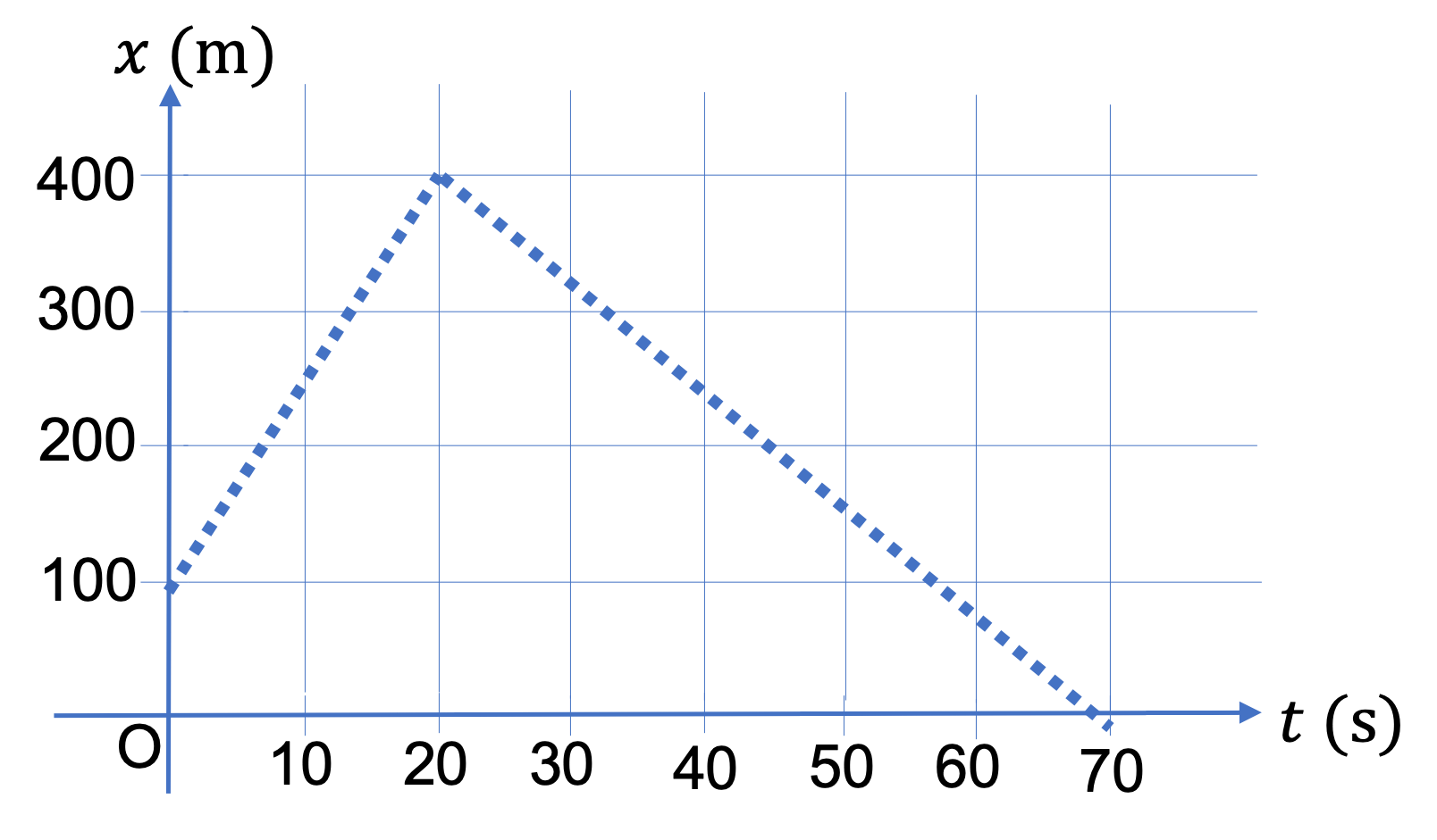
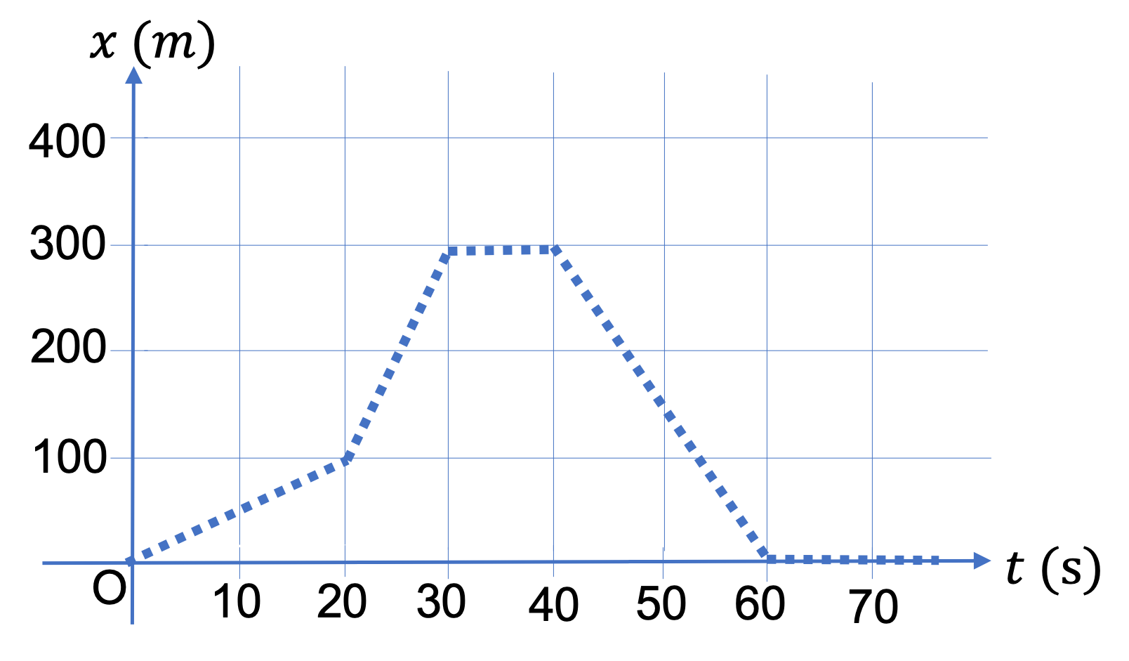
(a) Note that at \(t = 0 \text{,}\) the slope is not zero if we assume that the line contnues past \(t = 0 \) to the negative time. To determine \(v_x\) here, you read off two nearby points on the graph. For \(t = 0 \text{,}\) we will use \((t_1,x_1) = (0, 0) \) and \((t_2,x_2) = (20\text{ s}, 100\text{ m}) \text{.}\) From these we get \(v_x\) at \(t=0 \text{.}\)

\begin{equation*} v_x = \dfrac{x_2-x_1}{t_2-t_1} = \dfrac{100\text{ m} - 0}{20\text{ s} - 0} = 5.0\, \frac{\text{m}}{\text{s}}. \end{equation*}

(b) For \(t = 10 \) sec, we take points at \(t = 0 \) and \(t = 20 \) sec. We get the same value as in (a).

(c) For \(t = 25 \) sec, we take points at \(t = 20 \) sec and \(t = 30 \) sec, viz., \((t_1,x_1) = (20 \text{ s}, 100 \text{ m}) \) and \((t_2,x_2) = (30\text{ s}, 300 \text{ m}) \text{.}\) From these we get \(v_x\) at \(t = 25 \) sec.

\begin{equation*} v_x = \dfrac{x_2-x_1}{t_2-t_1} = \dfrac{300\text{ m} - 100\text{ m}}{30\text{ s} - 20\text{ s}} = 20.0\, \frac{\text{m}}{\text{s}}. \end{equation*}

(d) There is no change in \(x \) around this time point. So, \(v_x = 0\) at \(t = 35 \) sec.

(e) For \(t = 50 \) sec, we take points at \(t = 40 \) sec and \(t = 60 \) sec, viz., \((t_1,x_1) = (40 \text{ s}, 300 \text{ m}) \) and \((t_2,x_2) = (60\text{ s}, 0 ) \text{.}\) From these we get \(v_x\) at \(t = 50 \) sec.

\begin{equation*} v_x = \dfrac{x_2-t_2}{x_1-t_1} = \dfrac{0\text{ m} - 300\text{ m}}{60\text{ s} - 40\text{ s}} = -15.0\, \frac{\text{m}}{\text{s}}. \end{equation*}

Note that \(v_x \) here is negative. This is due to the fact that the train is moving in the same direction as the negative \(x \) axis.

(f) There is no change in \(x \) around this time point. Therefore, \(v_x = 0\) here.

Example 2.29. Velocity in Curved \(x \) vs \(t \) Graph.

The \(x \) coordinate of a runner plotted against time \(t \) as in the figure below.

We draw a tangent to the \(x \) versus \(t \) graph at the instant of interest, here \(t = 20 \) sec. The slope of the tangent line gives the numerical value of the \(x\)-velocity. Here \(x\)-velocity is positive since the runner’s \(x\) coordinate is increasing with time. That is, velocity has magnitude \(4.0\) m/s in the positive \(x\) direction.

You can see that the slope of the tangent has different values at different instants. Try looking at the slope at other times. This is a situation in which velocity \(v_x\) is changing with time. Can you find an instant when the \(x\)-velocity is zero in the figure? Hint: Look for a place where the tangent line is horizontal.

Subsection 2.4.5 Displacement from Velocity

Displacement is change in position during an interval. Suppose a motion is along \(x\)-axis with position \(x\) at instant \(t\) and \(x+\Delta x \) at instant \(t + \Delta t\text{.}\) Then, recall that average velocity for the finite interval \(t\) to \(t + \Delta t\) is given by

\begin{equation*} v_{x,av} = \frac{(x + \Delta x) - x}{ (t + \Delta t) - t} = \frac{\Delta x}{\Delta t}. \end{equation*}

Then, we can immediately get the displacement \(\Delta x\) by multiplying both sides by the interval \(\Delta t\text{.}\)

\begin{equation*} \Delta x = v_{x,av}\,\Delta t. \end{equation*}

How about getting the displacement \(\Delta x\) from instantaneous velocity \(v_x\) given at each instant between \(t\) and \(t + \Delta t\text{?}\) Since \(v_x\) is derivative of the function \(x(t)\text{,}\) to get change in \(x\text{,}\) we will need to integrate \(v_x\text{,}\) which is itself a function of \(t\text{.}\) Let us denote \(t_i\) for the intitial instant and \(t_f\) for the final instant, and \(x_f-x_i\) for \(\Delta x\text{.}\)

\begin{equation} v_x = \frac{dx}{dt}\ \ \longleftrightarrow\ \ x_f - x_i = \int_{t_i}^{t_f}\, v_x(t)\,dt.\tag{2.8} \end{equation}

Now, an integral has a nice graphical interpretation - it is the area "under or over" the curve! This is schematically illustrated in Fig. Figure 2.30

Figure 2.30. The area under the curve to get \(\Delta x \) from \(v_x\) versus \(t \) plot. The area for the curve when \(v_x \gt 0\) is positive, as between \(t=0 \) and \(t= 2\text{ sec}\) and the area for the curve when \(v_x \lt 0\) is negative, as between \(t= 2\text{ sec} \) and \(t= 4\text{ sec}\text{.}\)

Example 2.31. Displacement \(\Delta x\) from a \(v_x \) vs \(t \) Graph.

The instantaneous \(v_x \) of a car moving on a straight road is plotted against time \(t \) as shown in Figure 2.32. Find the displacements of \(x \) coordinate of the car during the following intervals of time:

(a) \(t = 0 \rightarrow 20 \text{ s}\text{,}\) (b) \(t = 20 \text{ s}\rightarrow 40 \text{ s}\text{,}\) and (c) \(t = 40 \text{ s}\rightarrow 70 \text{ s}\text{.}\)

Note that area can be negative here corresponding to \(x_f - x_i \lt 0 \text{.}\)

Answer.

(a) \(200\text{ m}\text{,}\) (b) 0, (c) \(-600\text{ m}\text{.}\)

Solution 1. a

We wish to find the area under the curve (which is a straight line here) between \(t = 0 \) and \(t = 20 \text{ s}\) - the shaded area in Figure 2.33. This is just the area of the triangle with base = 20 sec, and height = 20 m. Therefore,

\begin{equation*} x_f - x_i = \dfrac{1}{2} \times 20 \text{ m/s} \times 20 \text{ s} = 200 \text{ m}. \end{equation*}

Figure 2.33. Figure for Example 2.31, part (a).

Solution 2. b

We wish to find the area under the curve between \(t = 20 \text{ s} \) and \(t = 40 \text{ s}\) in Figure 2.34. This is sum of areas of two triangles, a triangle above the time axis (where \(v_x \gt 0 \)) and another below the time axis (where \(v_x \lt 0 \)). The area of the triangle with \(v_x \gt 0 \) will give positive area and the other one will give negative area. They happen to cancel out.

\begin{equation*} x_f - x_i = \dfrac{1}{2} \times 20 \text{ m/s} \times 10 \text{ s} + \dfrac{1}{2} \times (-20) \text{ m/s} \times 10 \text{ s} = 0\text{ m}. \end{equation*}

This means that the car went 100 m towards positive \(x \) axis and then backtracked same amount, ending up at the same \(x \) at the end as at the beginning.

Figure 2.34. Figure for Example 2.31, part (b).

Solution 3. c

We wish to find the area under the curve between \(t = 40 \text{ s} \) and \(t = 70 \text{ s}\) as shown in Figure 2.35. This is actually the area “above” the curve since the area of interest is the area between the curve and the abscissa of the plot.

\begin{equation*} x_f - x_i = \times (-20) \text{ m/s} \times 30 \text{ s} = -600\text{ m}. \end{equation*}

Figure 2.35. Figure for Example 2.31, part (c).

Exercises 2.4.6 Exercises

1. Average Velocity versus Average Speed.

A ball is rolling on a straight track. At the end of the track, the ball hits a wall and bounces back with the same speed. Ignore the time the ball was in contact with the wall during the collision. Let the original direction of ball be the positive \(x \) axis direction.

Let the ball be at \(x = 15\text{ cm}\) at \(t = 0 \text{,}\) and at \(x = 75\text{ cm}\) at \(t = 10\text{ sec} \text{.}\) The wall is at \(x = 100\text{ cm}\text{.}\) Suppose the collision occured sometime between \(t=0\) and \(t=10\text{ sec}\text{.}\)

What are (a) the average velocity and (b) average speed during the \(t = 0 \) to \(t = 10\text{ sec} \) interval?

Hint.

Average velocity on \(x\) axis is based on \(x\) coordinates and average speed is based on actual distance covered.

Answer.

(a) \(6 \text{ cm/s}\text{,}\) (b) \(11 \text{ cm/s}\text{.}\)

Solution 1. a

Average Velocity :

The definition of average velocity for a one-dimensional motion on \(x \) axis is

\begin{equation*} v_{\text{av},x} = \dfrac{\Delta x }{\Delta t}. \end{equation*}

Therefore,

\begin{equation*} v_{\text{av},x} = \dfrac{75\text{ cm} - 15\text{ cm}}{10\text{ sec}} = 6 \text{ cm/s}. \end{equation*}

Solution 2. b

Average Speed

The definition of average speed for any motion is

\begin{equation*} v_{\text{s,av}} = \dfrac{d }{\Delta t}. \end{equation*}

The motion has two legs here: (1) from \(x = 15\text{ cm} \) to \(x = 100\text{ cm} \) (i.e., the wall) and (2) from \(x = 100\text{ cm} \) to \(x = 75\text{ cm} \text{.}\) We need to add these distances, not just difference in coordinates. Therefore,

\begin{equation*} v_{\text{s,av}} = \dfrac{85\text{ cm} + 25\text{ cm}}{10\text{ sec}} = 11 \text{ cm/s}. \end{equation*}

2. Compute \(\Delta x \) from \(v_x \) versus \(t \) plot.

From the \(v_x \) versus \(t \) plot in Figure 2.37, find change in \(x \) during the following intervals given in seconds (a) \((0, 2) \text{,}\) (b) \((2, 3) \text{,}\) (c) \((3, 4) \text{,}\) and (d) \((0, 4) \text{.}\)

Figure 2.37. Figure for Exercise 2.4.6.2.

Hint.

Use areas.

Answer.

(a) \(8\text{ m}\text{,}\) (b) \(2\text{ m}\text{,}\) (c) \(-1\text{ m}\text{,}\) (d) \(9\text{ m}\text{.}\)

Solution 1. a

This is a rectangular area, of height \(4\text{ m/s}\) and width \(2\text{ sec}\text{.}\) The line is above the \(v_x = 0 \) line. Therefore, the change in \(x \) will be:

\begin{equation*} \Delta x = 4\text{ m/s} \times 2\text{ s} = 8\text{ m}. \end{equation*}

Solution 2. b

(b) This is triangular area, of height \(4\text{ m/s}\) and base \(1\text{ sec}\text{.}\) The line is above the \(v_x = 0 \) line. Therefore, the change in \(x \) will be:

\begin{equation*} \Delta x = \dfrac{1}{2}\times 4\text{ m/s} \times 1\text{ s} = 2\text{ m}. \end{equation*}

Solution 3. c

This is triangular area, of height \(2\text{ m/s}\) and base \(1\text{ sec}\text{.}\) The line is below the \(v_x = 0 \) line. Therefore, the change in \(x \) will be:

\begin{equation*} \Delta x = -\dfrac{1}{2}\times 2\text{ m/s} \times 1\text{ s} = -1\text{ m}. \end{equation*}

Solution 4. d

(d) This is just the sum of all the areas in (a), (b), and (c).

\begin{equation*} \Delta x = 8\text{ m} + 2\text{ m} -1\text{ m} = 9\text{ m}. \end{equation*}

3. Displacement from \(v_x \) vs \(t \) Graph.

The \(v_x \) of a car moving on a straight road is plotted against time \(t \) as shown in Figure 2.38. Find the displacements of the car during the following intervals of time: (a) \(t = 0 \rightarrow 20 \text{ s}\text{,}\) (b) \(t = 20 \text{ s}\rightarrow 40 \text{ s}\text{,}\) (c) \(t = 40 \text{ s}\rightarrow 50 \text{ s}\text{,}\) (d) \(t = 50 \text{ s}\rightarrow 70 \text{ s}\text{,}\) and (e) \(t = 10 \text{ s}\rightarrow 20 \text{ s}\text{.}\)

Figure 2.38. Figure for Exercise 2.4.6.3.

Hint.

Find the areas between the plot line and the time axis.

Answer.

(a) \(200 \) m, (b) \(200 \) m, (c) \(-50 \) m, (d) \(-200\) m, (e) \(150\) m.

Solution 1. a

The area under the plot (or, over the plot if \(v_x \lt 0\)) is the displacement. We use area of triangle = \(\dfrac{1}{2} \times \) base \(\times \) height and area of a rectangle = base \(\times \) height.

\(\Delta x = 0.5 \times 20 \text{ s} \times 20 \text{ m/s} = 200 \text{ m}.\)

Solution 2. b

\(\Delta x = 0.5 \times 20 \text{ s} \times 20 \text{ m/s} = 200 \text{ m}.\)

Solution 3. c

\(\Delta x = 0.5 \times 10 \text{ s} \times (-10 \text{ m/s} ) = -50 \text{ m}.\)

Solution 4. d

\(\Delta x = 20 \text{ s} \times (-10 \text{ m/s} ) = -200 \text{ m}.\)

Solution 5. e

This one is different - here we need to add two parts, one a triangle and the other a square.

\(\Delta x = 0.5 \times 10 \text{ s} \times 10 \text{ m/s} + 10 \text{ s} \times (10 \text{ m/s} ) = 150 \text{ m}.\)

4. Velocity from Position Given as a Function of Time.

The position of a box sliding in a straight line is given by the

-coordinate of one of its corners. It is found that, while the \(y\) and \(z\)-coordinates do not change, the \(x\)-coordinate varies as a function of time \(t\) as

\begin{equation*} x(t) = 4 + 18 t - 5 t^2, \end{equation*}

where \(t\) is in seconds and \(x\) in meters.

(a) Determine the instantaneous velocity and speed of the box at following instants in time. (i) \(t = 0\text{,}\) (ii) \(t = 1\) sec, (iii) \(t = 2\) sec, and (iv) \(t = 3\) sec.

(b) Find the average velocity of the box during the following intervals. (i) \([0, 1\ \text{s}]\text{,}\) (ii) \([0, 2\ \text{s}]\text{,}\) (iii) \([1\ \text{s}, 2\ \text{s}]\text{,}\) (iv) \([0, 3\ \text{s}]\text{,}\) and (v) \([1\ \text{s}, 3\ \text{s}]\text{.}\)

Hint.

Take derivative and evaluate at given instants.

Answer.

See solution.

Solution 1. a

Since the \(x\) coordinate of the particle is given as a function of \(t\) we can determine the \(x\)-component of the velocity by calculating the derivative.

\begin{equation*} v_x(t) = \frac{dx}{dt} = \frac{d}{dt} \left(4 + 18 t - 5 t^2\right) = 18 - 10 t. \end{equation*}

The \(x\)-component of the instantaneous velocity at different instants is obtained by plugging values of \(t\) for those instants. We find the following for the velocities at the instants in question.

\begin{align*} \amp \text{(i) } v_x(0) = 18\ \text{m/s}. \\ \amp \text{(ii) } v_x(1 s)= 8\ \text{m/s}.\\ \amp \text{(iii) } v_x(2 s) = -2\ \text{m/s}.\\ \amp \text{(iv) } v_x(3 s) = -12\ \text{m/s}. \end{align*}

Solution 2. b

The average velocity in time interval, as opposed to the instantaneous velocity at one instant, is calculated from the change in the position over that interval. Here, the \(x\)-component of the average velocity in an interval \(t_1\) to \(t_2\) is obtained by

\begin{equation*} v_x^{\text{ave}} = \frac{x(t_2)-x(t_1)}{t_2-t_1}. \end{equation*}

Since the \(y\)- and \(z\)-components of the average velocity are zero here, the average velocity is

\begin{equation*} \vec v_{\text{ave}} = v_x^{\text{ave}} \hat u_x. \end{equation*}

To start with we need the \(x\) coordinates at \(t = 0\text{,}\) \(t = 1\) s, \(t = 2\) s, and \(t = 3\) s. These values are: \(x(0) = 4\ \text{m}\text{,}\) \(x(1\ \text s) = 17\ \text{m}\text{,}\) \(x(2\ \text s) = 20\ \text{m}\text{,}\) and \(x(3\ \text s) = 13\ \text{m}\text{.}\) Using these values we find the velocities in the intervals asked in the question.

(i) \([0, 1\ \text{s}]\text{:}\)

\begin{align*} \amp v_x = \frac{x(1\ \text s) - x(0)}{1\ \text s-0} = \frac{17\ \text{m} - 4\ \text{m}}{1\ \text s} = 13\frac{\text{m}}{\text s}. \end{align*}

(ii) \([0, 2\ \text{s}]\text{:}\)

\begin{align*} \amp v_x = \frac{x(2\ \text s) - x(0)}{2\ \text s-0} = \frac{20\ \text{m} - 4\ \text{m}}{2\ \text s} = 8\frac{\text{m}}{\text s}. \end{align*}

(iii) \([1\ \text{s}, 2\ \text{s}]\text{:}\)

\begin{align*} \amp v_x = \frac{x(2\ \text s) - x(1\ \text s)}{2\ \text s-1\ \text s} = \frac{20\ \text{m} - 17\ \text{m}}{1\ \text s} = 3\frac{\text{m}}{\text s}. \end{align*}

(iv) \([1\ \text{s}, 3\ \text{s}]\text{:}\)

\begin{align*} \amp v_x = \frac{x(3\ \text s) - x(1\ \text s)}{3\ \text s-1\ \text s} = \frac{13\ \text{m} - 17\ \text{m}}{2\ \text s} = -2\frac{\text{m}}{\text s}. \end{align*}

5. (Calculus) Velocity from Derivative.

A block of copper attached to a spring executes a one-dimensional motion. The position of the center of the block varies with time according to the following function, \(x(t) = 5.0\ \cos(2\pi t/T)\text{,}\) where \(t \) is in sec, \(T=1\text{ sec}\) and \(x \) in cm. The argument of cosine is radians not degrees.

(a) Determine the instantaneous velocity and speed at the following instants: (i) \(t = 0\text{,}\) (ii) \(t = 1/4\text{ sec}\text{,}\) (iii) \(t = 1/2\text{ sec}\text{,}\) (iv) \(t = 3/4\text{ sec}\text{,}\) (v) \(t = 1.0\text{ sec}\text{,}\) (vi) \(t = 3/2\text{ sec}\text{.}\)

(b) Find the average velocities in the following intervals. (i) \([0, 1/4\text{ sec}]\text{,}\) (ii) \([1/4\text{ sec}, 1/2\text{ sec}]\text{,}\) (iii) \([0, 1/2\text{ sec}]\text{,}\) (iv) \([0, 1 \text{ sec}]\text{,}\) and (v) \([0, 3/2 \text{ sec}]\text{.}\)

Hint.

(a) Take derivative and evaluate at the instants. (b) Evaluate \(\Delta x\) for the intervals.

Answer.

(a) \(0.0, -31.4\text{ cm/s}. 0.0, 31.4 \text{ cm/s}, 0.0, 0.0 \text{.,}\) (b) \(-20.0\text{ cm/s}, -20.0\text{ cm/s}, -20.0\text{ cm/s}, 0.0, -6.66\text{ cm/s} \text{.}\)

Solution 1. a

Let us find \(v_x\) at arbitrary instant \(t\) by taking the derivative of \(x\text{.}\) In units \(\text{m/s}\) we get

\begin{equation*} v_x = \dfrac{dx}{dt} = -10.0\,\pi \sin(2\pi t). \end{equation*}

Evaluating at instants asked give the following values.

\(\displaystyle 0.0,\)
\(\displaystyle -31.4 \text{ cm/s},\)
\(\displaystyle 0.0,\)
\(\displaystyle 31.4 \text{ cm/s},\)
\(\displaystyle 0.0,\)
\(\displaystyle 0.0.\)

Instanteous speeds at these instants are obtained from absolute values of \(v_x\) here, with values \(0,\ 31.4\text{ cm/s},\ 0, 31.3\text{ cm/s},\ 0, \ 0\text{.}\)

Solution 2. b

The average velocity between two instants, \(t=t_1\) and \(t=t_2\) will be

\begin{equation*} v_{\text{av},x} = \dfrac{ x(t_2) - x(t_1) }{t_2 - t_1}. \end{equation*}

We need positions at various instants. They are

\begin{align*} \amp x(0) = 5\text{ cm},\ \ x(0.25\text{ s}) = 0,\ \ x(0.5\text{ s}) = -5\text{ cm},\\ \amp x(1) = 5\text{ cm}, \ \ x(1.5\text{ s}) = -5\text{ cm}. \end{align*}

Using these values we get average velocities to be:

\(\displaystyle -20.0 \text{ cm/s},\)
\(\displaystyle -20.0 \text{ cm/s},\)
\(\displaystyle -20.0 \text{ cm/s},\)
\(\displaystyle 0.0,\)
\(\displaystyle -6.67\text{ cm/s}.\)

6. (Calculus) Determining \(\Delta y\) from Given \(v_y(t)\).

The \(y\)-velocity of a parchute jumper is given by

\begin{equation*} v_y = v_0 \left( 1 - e^{-\alpha t} \right), \end{equation*}

where \(v_0\) and \(\alpha\) are constant. What is the change in \(y\) during interval \(t=0\) to \(t=T\text{?}\)

Hint.

Integrate \(v_y\text{.}\)

Answer.

\(v_0 T + \dfrac{v_0}{\alpha} \left( e^{-\alpha T} - 1\right)\text{.}\)

Solution.

Integrating \(v_y\) will give us the answer.

\begin{align*} \Delta y \amp = \int_0^T v_y\, dt, \\ \amp = \int_0^T v_0 \left( 1 - e^{-\alpha t} \right) \, dt, \\ \amp = v_0 T + \dfrac{v_0}{\alpha} \left( e^{-\alpha T} - 1\right). \end{align*}

7. (Calculus) Practice with a Friend.

A ball is shot straight up with speed \(v_0\text{.}\) Let positive \(y\) axis be pointed up. Using this coordinate system, you find that its velocity is changing with time according to the following equation.

\begin{equation*} v_y = v_0 - g t, \end{equation*}

where \(g\) is a constant. Find the position of the ball at some arbitrary instant, \(t=T\text{.}\)

Hint.

Integrate \(v_y\text{.}\)

Answer.

\(v_0 T - \frac{1}{2} g T^2\text{.}\)

Prev Top Next