
Section 41.7 Faraday's Law

(Calculus) EMF and Nonconservative Electric Field.

EMF in a circuit is the net work done by the driving force per unit charge in the circuit. The driving force in a circuit must come from electric field since magnetic force on a moving charge is perpendicular to velocity, and hence, can do no work.

Since electric field is equal to the force per unit charge, the induced EMF will be equal to the line integral of the electric field around the circuit. The line integral calculated in the direction of the electric field gives a positive value for the EMF. The closed line integral is indicated by placing a circle on the symbol of the integral as before.

\begin{equation} \mathcal{E}_\text{ind} = \oint_\text{closed loop}\vec E_\text{ind}\cdot d\vec l. \label{eq-induced-emf-from-line-integral}\tag{41.7.1} \end{equation}

In static electricity we had learned that potential difference between two points A and B is also a line integral of electric field, viz.,

\begin{equation*} \phi_B - \phi_A = - \int_A^B\, \vec E_\text{static}.d\vec l. \end{equation*}

In a closed path, A and B will be same point, so, we would get

\begin{equation} \oint_\text{closed path}\, \vec E_\text{static}.d\vec l = 0.\label{eq-static-conservative-field-Kirchoff}\tag{41.7.2} \end{equation}

That is, \(\vec E_\text{static}\) was a conservative field. This equation was the basis of Kirchoff's voltage law (KVL).

But, in the case of dynamical electric field of Eq. (41.7.1), the line integral around a closed path is not zero. We say that dynamically generated electric field is non-conservative field. Let us denote this field by emphasizing it to be dynamic. Thus, we can say that

\begin{equation} \oint_\text{closed path}\, \vec E_\text{dynamic}.d\vec l \ne 0.\label{eq-dynamic-conservative-field-Kirchoff}\tag{41.7.3} \end{equation}

The non-zero result is the induced EMF in the circuit. Since dynamic electric field violates Kirkchoff's voltage rule, we cannot use Kirkchoff's voltage rule when we are working with dynamic nonconservative electric field. Instead, we must use Faraday's law as given in Subsection 41.7.1 below.

Subsection 41.7.1 (Calculus) Faraday's Law

We find that EMF in a circuit is

\begin{equation*} \mathcal{E}_\text{ind}(t) = \oint_{\text{closed loop, L(t)}} \vec E\cdot d\vec l. \end{equation*}

If magnetic flux is changing in a circuit, then EMF must equal

\begin{equation*} \mathcal{E}_\text{ind}(t) = -\dfrac{d\Phi_B}{dt}, \end{equation*}

where \(\Phi_B\) is magnetic flux, which is an integral over the area enclosed by the circuit.

\begin{equation*} \Phi_B = \iint_{\text{Loop surface, S(t)}} \vec B\cdot d\vec A, \end{equation*}

where I have indicates that loop surface, itself may be changing with time, by using symbol \(S(t)\) for the surface. Putting the two expressions of EMF of a circuit, we get integral form of Faraday's law.

\begin{equation} \oint_{\text{closed loop, L(t)}} \vec E\cdot d\vec l = -\dfrac{d}{dt}\iint_{\text{open surface, S(t)}} \vec B\cdot d\vec A.\label{eq-faraday-law-general}\tag{41.7.4} \end{equation}

The minus sign in Eq. (41.7.4) is needed to give the correct direction of the induced EMF in the circuit when the integral is conducted in the direction of the electric field and the right-hand illustrated in the figure is used for the direction of the area vector.

Note that the time derivative on the right side of Eq. (41.7.4) is outside the integral whose limits may be functions of time if the surface attached to the loop changes with time, as would be the case if shape of the loop changing in time. The derivative of the parameters that define the attached surface gives the contribution of the magnetic force on the conductor at the boundary. That means, we have included EMF from both the flux rule and Lorentz law.

Another aspect of Faraday's law worth noting is that the relation between the electric and magnetic fields given by the Faraday's law applies to any loop in space whether or not the points on the loop are occupied by a physical wire since we do no need to worry about induced current. If we have a conducting wire for the loop, we have induced current in the conductor. In that case, the magnetic flux, will be flux of net magnetic field, i.e., the flux of external as well as induced magnetic field.

The Faraday's law says that magnetic field and electric field are intimately connected to each other - a changing magnetic field gives rise to an electric field. You might wonder if a changing electric field will similarly give rise to a magnetic field. So far we have seen that only magnets and electric currents create magnetic field. Maxwell showed that a changing electric field also gives rise to a magnetic field which we will study in a later chapter.

Subsection 41.7.2 Analogy Between Faraday's law and Ampere's law

The problem of magnetic field of steady currents and the problem of electric field from changing magnetic fluxhere are completely analogous mathematically if there are no charges around as seen from the following equations.

\begin{align*} \text{Magnetic field} \amp \ \text{of steady current:}\\ \amp \oint \vec B\cdot d\vec A = 0\ \ \ \text{(since no magnetic charges)}\\ \amp \oint \vec B\cdot d\vec l = \mu_0 I_\text{enc} \end{align*}
\begin{align*} \text{Electric field}\amp \ \text{with no charges:}\ \ \\ \amp \oint \vec E\cdot d\vec A = 0\ \ \ \text{(since no electric charges)}\\ \amp \oint \vec E\cdot d\vec l = -\dfrac{d\Phi_B}{dt}. \end{align*}

This suggests that the problem-solving techniques of Ampere's law can be fruitfully employed by recognizing that \(-d\Phi_B/dt\) of a Faraday's law problem corresponds to \(\mu_0 I_\text{enc}\) in the corresponding Ampere's law problem. I will present an example below that makes the use of this mathematical analogy to deduce the electric field from a changing magnetic field.

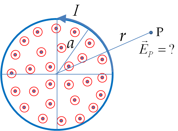
A long cylindrical solenoid of radius \(a\) having \(n\) turns per unit length carries a time-dependent current \(I(t)\text{.}\) Find electric field at a point P outside the solenoid as shown in figure, where, for the sake of clarity, only a cross-section of the solenoid is shown.

Figure 41.7.2. Checkpoint 41.7.1.
Hint

Study the solution.

Answer

See solution.

Solution

Recall that the current in a solenoid produces a uniform magnetic field inside the solenoid of the magnitude \(\mu_0 n I\) and zero outside the solenoid. The direction of the magnetic field depends on the current direction given by the right-hand rule of Biot-Savart's law: if you look down the axis, then the direction of magnetic field will be towards you if the current loops around in a counter-clockwise direction as given in the problem statement.
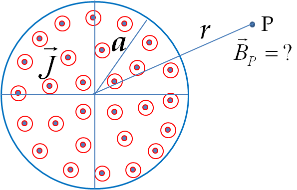
From the analogy of Ampere's law and Faraday's law discussed above, we note that the problem here is analogous to the Ampere's law problem of finding magnetic field outside a straight wire that carries a uniform volume current density \(\vec J\) as shown in the figure.

Therefore, in the present situation we can claim that the electric field will circulate in circles around the magnetic field just as the magnetic field of a straight wire circulates around the current. Following the Ampere's law procedure for a straight wire, we choose an “Amperian loop” in the shape of a circle that passes through the field point P as shown in Figure 41.7.3. Now, we equate the circulation of electric field around the Amperian loop with the “enclosed” rate of change of magnetic flux through the Amperian loop.

\begin{equation*} \text{Circulation of }\vec E = - \text{ Enclosed rate of change of magnetic flux.} \end{equation*}

Since the electric field has the same amplitude at all points of the circle the circulation is just a product of the amplitude of the electric field and circumference of the circle of radius \(r\text{,}\) which is the distance of field point P from the axis of solenoid. The enclosed magnetic flux is also easy to calculate here since the magnetic field is zero outside the solenoid.

Figure 41.7.3. The Amperian loop passes through the field point and the magnetic flux is calculated over the area enclosed by the Amperian loop shown shaded here. The direction of the Amperian loop and area vector are related by the right-hand rule. Although there is no magnetic field at P, there is an electric field there due to the changing magnetic field inside the solenoid.

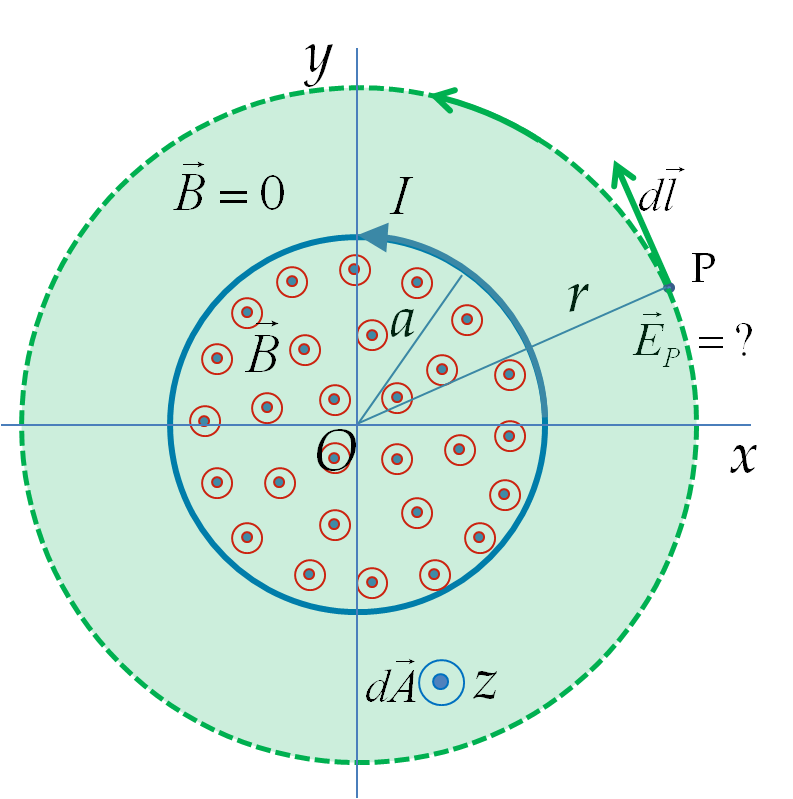
To include the direction information, we cast the circulation and magnetic flux in terms of components. The right-hand rule for Faraday's law shows that, if the direction of the loop for the circulation is taken along \(\hat u_{\phi}\text{,}\) then the direction of the area element will be towards the positive \(z\)-axis as shown in Figure 41.7.3. This will give the following for the \(\phi\)-component of electric field.

\begin{equation*} \left(2\pi r\right) E_{\phi} = -\left( \mu_0 \dfrac{dI}{dt} n \right) \left( \pi a^2\right), \end{equation*}

where the minus sign on the right side comes from the minus sign in the Faraday's law. Solving for \(E_{\phi}\) we find

\begin{equation*} E_{\phi} = -\dfrac{\mu_0 n a^2}{2r}\dfrac{dI}{dt}. \end{equation*}

Therefore, the electric field induced at a point P outside the solenoid is

\begin{equation*} \vec E_P = -\dfrac{\mu_0 n a^2}{2r}\dfrac{dI}{dt} \hat u_{\phi}. \end{equation*}

We find that the induced electric field at the space point P circulates clockwise for an increasing current \((dI/dt>0)\) and counter-clockwise for a decreasing current \((dI/dt\lt 0)\text{.}\) If you place a circular metal wire of radius \(r\) which coincides with the Amperian loop for the circulation of \(\vec E\) calculation, you will notice that there is an induced current in the direction of the induced electric field. Also, if you place a charge anywhere outside the solenoid, the charge will experience an electric force in the axial direction when the current in the solenoid is changing, but no such force when the current in the solenoid is steady.

The result obtained here implies a rather strange conclusion: the electric field at a point outside of a solenoid with a time-varying current is not zero, although the magnetic field there is zero! Note that this takes place only when the current in the solenoid is changing; once the current has become steady, there would be no electric field outside the solenoid.

Electric field inside solenoid

To find electric field induced at a point inside the solenoid we will choose Amperian loop with radius \(r\lt a\) as shown in Figure 41.7.4.

Figure 41.7.4. The Amperian loop and are enclosed (shaded) for a point inside the solenoid.

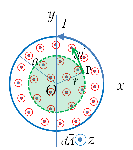
The enclosed magnetic flux will be less than the flux through the entire cross-section of the solenoid - instead, the magnetic flux through only an area \(\pi r^2\) will be enclosed within the Amperian loop. This gives the electric field that increases with the distance from the axis inside the solenoid.

\begin{equation*} \vec E_P = -\dfrac{\mu_0 n r}{2}\dfrac{dI}{dt} \hat u_{\phi}\ \ \text{(at a point P inside)}. \end{equation*}

The current in a long solenoid of radius 3 cm and 25 turns/cm is varied with time at a rate of 2 A/s. Find the electric field at a distance 4 cm from the center of the solenoid.

Hint

Use “Ampere's law” for dynamic \(E\) field.

Answer

\(3.33\times 10^{5} \ \textrm{N/C}\text{.}\)

Solution

From Faraday law, we have

\begin{equation*} \oint\:\vec E\cdot d\vec l = \mathcal{E} = \dfrac{d\Phi}{dt}. \end{equation*}

Here \(\dfrac{d\Phi}{dt}\) has a cylindrical symmetry. Hence, we can use “Ampere's Law” type of arguments to assert that the electric field will circulate around the solenoid. Hence the electric field at a distance \(r\) from the axis of the solenoid will obey

\begin{equation*} 2\pi r\times E = \mathcal{E}\ \ \Longrightarrow\ \ E = \dfrac{\mathcal{E}}{2\pi r}. \end{equation*}

Putting in the expression for \(\Phi\) for a solenoid n we find

\begin{align*} E \amp = \dfrac{\mu_0\:n\:\Delta I/\Delta t}{2\pi r} \\ \amp = \dfrac{4\pi\times 10^{-7}\times 2500\times 2}{2\pi \times 0.03} = 3.33\times 10^5\:\textrm{N/C}. \end{align*}