Displacement from Velocity

Section 4.5 Displacement from Velocity

Recall that velocity \(\vec v\) is derivative of position \(\vec r\text{.}\) To emphasize that this definition is true at each instant \(t\text{,}\) let us write each vector with its dependence on time \(t\text{.}\)

\begin{equation} \vec v(t) = \frac{d\vec r(t)}{dt}.\tag{4.32} \end{equation}

Now, we ask how can we get dispacement, i.e., change in position in an interval \(t=t_i\) to \(t=t_f\text{?}\) From Calculus, this is obtained by integrating both sides of this equation from \(t=t_i\) to \(t=t_f\text{.}\) Formally, the steps of calculation would go as follows.

\begin{equation} \int_{t_i}^{t_f}\vec v(t) dt = \int_{t_i}^{t_f} \frac{d\vec r(t)}{dt} dt.\tag{4.33} \end{equation}

The canceling \(dt\) on the right side, gives integral over \(d\vec r\text{,}\) which leads to just change in position when integrated.

\begin{equation} \int_{t_i}^{t_f} \frac{d\vec r(t)}{dt} dt = \int_{\vec r_i}^{\vec r_f} \frac{d\vec r(t)} = \vec r_f - \vec r_i.\tag{4.34} \end{equation}

That is, displacment in the time interval is given by the integration of the velocity vector over that interval.

\begin{equation} \vec r_f - \vec r_i = \int_{t_i}^{t_f}\vec v(t) dt.\tag{4.35} \end{equation}

The components of this equation are related to integrating the components of the velocity.

\begin{align} \amp x_f - x_i = \int_{t_i}^{t_f}v_x(t) dt \tag{4.36}\\ \amp y_f - y_i = \int_{t_i}^{t_f}v_y(t) dt \tag{4.37}\\ \amp z_f - z_i = \int_{t_i}^{t_f}v_z(t) dt \tag{4.38} \end{align}

In this form, since we are dealing with integration over ordinary functions, and nor a vector fuction of \(t\text{,}\) we can interpret the right sides of these component equations in terms of area under the curve or area above the curve in a plot of the correponding velocity component.

That is, if you plot \(v_x\) versus \(t\text{,}\) the right side of equation (4.36) can be evaluated by the integration below the plot if \(v_x\) is positive in the time range and above the plot if \(v_x\) is negative with area now negative. The sum of all positive and negative areas in the interval will give \(\Delta x \equiv x_f - x_i\text{.}\) Similarly, for \(\Delta y\) and \(\Delta z\text{.}\)

Example 4.51. Area Under the Velocity versus Time Plot.

To interpret Eqs. (4.36) , let us look at a numerical example where \(v_x\) is constant. Then, integration gives

\begin{equation*} \int_{t_i}^{t_f}v_x(t) dt = v_x \int_{t_i}^{t_f} dt = v_x( t_f - t_i ) = v_x\, \Delta t. \end{equation*}

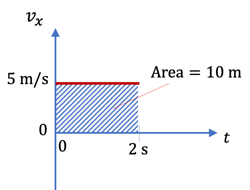
Let \(v_{x} = 5\text{ m/s}\) and \(\Delta t = 2\text{ s}\text{.}\) Suppose we plot \(v_x \) versus \(t\text{,}\) then we will find that \(v_{x}\times {\Delta t} = 10 \text{ m}\) gives us the area under the \(v_x \) versus \(t\) plot, which is equal to change in \(x\text{,}\) \(\Delta x = 5\text{ m/s} \times 2\text{ s} = 10 \text{ m}\text{.}\)

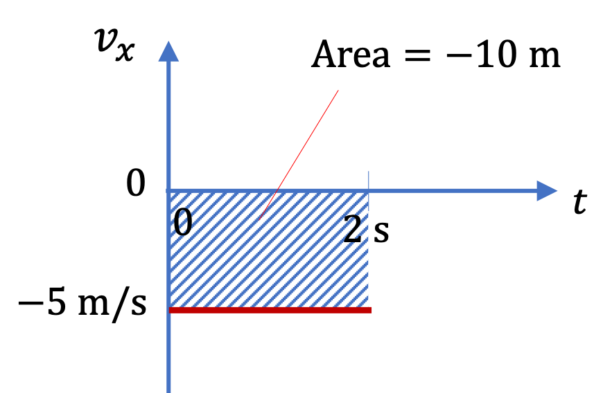
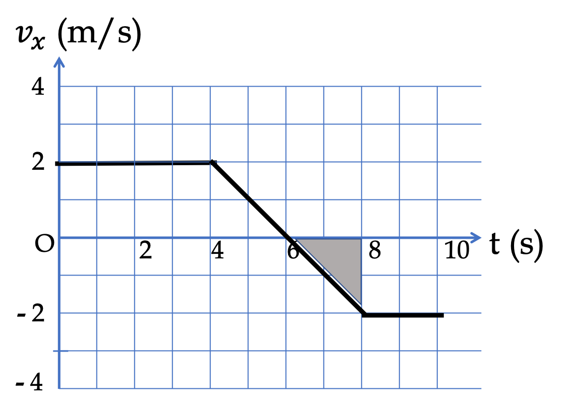
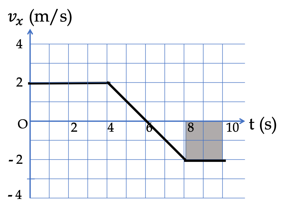
If velocity \(v_x\) is negative during the interval, it would mean that object is moving towards negative \(x\) axis. This shows up as negative area above the plot. Therefore, the \(x\) displacement will be \(\Delta x = -5\text{ m/s} \times 2\text{ s} = - 10 \text{ m}\text{.}\)

Example 4.52. Displacement from Velocity - Areas Under Curve.

Figure 4.53 shows a \(v_x \) versus \(t\) plot. Find the displacements in the following intervals, given in seconds, (a) \((0,\ 4)\text{,}\) (b) \((4,\ 6)\text{,}\) (c) \((6,\ 8)\text{,}\) (d) \((8,\ 10)\text{,}\) and (e) \((0,\ 10)\text{.}\)

Answer.

(a) \(8\text{ m}\text{,}\) (b) \(2\text{ m}\text{,}\) (c) \(-2\text{ m}\text{,}\) (d) \(-4\text{ m}\text{,}\) (e) \(4\text{ m}\text{.}\)

Solution 1. a

Note that the \(t \) axis is the \(v_x = 0 \) line. Therefore, we need the area of the shaded region in the figure on the right. This gives

\begin{align*} \Delta x \amp = 4\text{ s} \times 2\text{ m/s}\\ \amp = 8\text{ m}. \end{align*}

Solution 2. b

Note that the \(t \) axis is the \(v_x = 0 \) line. Therefore, we need the area of the shaded region in the figure on the right. This gives

\begin{equation*} \Delta x = \dfrac{1}{2}\times 2\text{ s} \times 2\text{ m/s} = 2\text{ m}. \end{equation*}

Solution 3. c

Note that the \(t \) axis is the \(v_x = 0 \) line. Therefore, we need the area of the shaded region in the figure on the right. This area will be negative as is also clear from the direction motion - it is moving to the left. This gives

\begin{align*} \Delta x \amp = \dfrac{1}{2}\times 2\text{ s} \times (-2\text{ m/s})\\ \amp = -2\text{ m}. \end{align*}

Solution 4. d

\begin{align*} \Delta x \amp = 2\text{ s} \times (-2\text{ m/s})\\ \amp = -4\text{ m}. \end{align*}

Solution 5. e

Adding up all the areas we get

\begin{equation*} \Delta x(0\rightarrow 10\text{ s}) = 8\text{ m} + 2\text{ m} + (-2)\text{ m} + (-4)\text{ m} = 4\text{ m}. \end{equation*}

Example 4.54. (Calculus) Displacement from Velocity.

A particle is moving in a circle with its velocity components changing with time as given by (in units of m/s with \(t\) in units of seconds.)

\begin{equation*} v_x = 5.0\,\cos(2\pi t),\ \ \ v_y = 5.0\,\sin(2\pi t)\text{.} \end{equation*}

(a) What are the components of the displacement vector during the interval from \(t=0.25\text{ s} \) to \(t=0.50\text{ s} \text{.}\) (b) What are the magnitude and direction of the displacement?

Answer.

(a) \((-0.80\text{ m},\ 0.80\text{ m} ) \) (b) \(1.13\text{ m} \) in \(45^{\circ} \) direction from the negative \(x \) axis into the second quadrant.

Solution 1. a

The components will be obtained by taking the integral.

\begin{align*} \Delta x \amp = \int_{0.25}^{0.5}\, 5.0\,\cos(2\pi t)\, dt, \\ \amp = \dfrac{5.0}{2\pi}\sin(2\pi t)|_{0.25}^{0.5} \\ \amp = -0.80\text{ m}. \end{align*}

\begin{align*} \Delta y \amp = \int_{0.25}^{0.5}\, 5.0\,\sin(2\pi t)\, dt, \\ \amp = -\dfrac{5.0}{2\pi}\cos(2\pi t)|_{0.25}^{0.5} \\ \amp = 0.80\text{ m}. \end{align*}

Solution 2. b

Therefore, the magnitude and angle will be:

\begin{gather*} \Delta r = 0.8\times \sqrt{2} = 1.13\text{ m},\\ \theta = \tan^{-1}(-1) = - 45^{\circ}, \end{gather*}

which we interpret to be clockwise angle of \(45^{\circ} \) from the negative \(x \) axis into the second quadrant.

Exercises Exercises

1. Change in \(x\)-coordinate from Constant \(v_x\).

A ball is rolling on the floor such that its \(x\)-coordinate in a particular Cartesian coordinate system changes at a constant rate \(u_0\text{.}\) If the \(x\)-coordinate is \(x_0\) at \(t=t_0\) what will be the \(x\)-coordinate at \(t=T\text{?}\)

Solution.

From our discussion we know that the rate of change in a coordinate is given by the derivative of the coordinate with time.

\begin{equation*} \frac{dx}{dt} = \textrm{Rate of change of } x \textrm{ coordinate}. \end{equation*}

Here the rate is given to be \(u_0\text{.}\) Therefore, we have the following equation for the derivative of \(x(t)\text{.}\)

\begin{equation*} \frac{dx}{dt} = u_0. \end{equation*}

This equation can also be written for differential elements, \(dx\) and \(dt\) by multiplying both sides by \(dt\text{.}\)

\begin{equation*} dx = u_0dt, \end{equation*}

which we can integrate on both sides. On the left side, the limit of integration is \(x_0\) to \(x(T)\) and the limit on the right side is the times for those \(x\) values, viz. from \(t_0\) to \(T\text{.}\)

\begin{equation*} \int_{x_0}^{x(T)}dx = \int_{t_0}^{T}u_0dt, \end{equation*}

which gives the following result.

\begin{equation*} x(T) - x_0 = u_0(T-t_0). \end{equation*}

Further Observations:

An integration is actually not necessary here since the rate of change is constant in time. The constant rate implies that the average rate is the same as instantaneous rate of change. Therefore,

\begin{equation*} \frac{\Delta x}{\Delta t} = u_0, \end{equation*}

which can be multiplied both sided by \(\Delta t\) to solve for \(\Delta x\text{.}\) This immediately gives the change over the interval from \(t_0\) to \(T\) as

\begin{equation*} x(T) - x_0 = u_0(T-t_0). \end{equation*}

2. Change in \(x\)-coordinate from Varying \(v_x\).

A particle moves in the \(xy\)-plane of a coordinate system. The rate of change of its \(x\)-coordinate varies linearly with time such that the rate at any particular time is \(v_x = u_0 + b t^2\text{,}\) where \(u_0\) and \(b\) are constants. If the \(x\)-coordinate is \(x_0\) at \(t=t_0\) what will be the \(x\)-coordinate at \(t=T\text{?}\)

Solution.

The discussion of the last example takes us to the following equation for the differentials

\begin{equation*} dx = \left(u_0 + b t^2\right)dt, \end{equation*}

which can be integrated to give

\begin{equation} x(T) - x_0 = u_0(T-t_0) + \frac{b}{3}\left( T^3-t_0^3 \right).\tag{4.39} \end{equation}

Further Observations:

Here we must resort to integration since the rate is changing with time. The short-cut method applicable for constant rate does not give the correct answer. The average rate is also not equal to the average of the \(x\)-component of velocity at the end and the \(x\)-component of velocity at the beginning.

\begin{equation*} v_{av,x} \ne \frac{v_x(T) + v_x(t_0)}{2}. \end{equation*}

The \(x\)-component of the average velocity is equal to the change in the \(x\)-coordinate divided by the interval. Using Eq. (4.39) we find \(v_{ave}\) to be

\begin{equation*} v_{av,x} = \frac{x(T) - x_0}{T - t_0} = u_0 + \frac{b}{3}\left( T^2 + t_0T + t_0^2\right), \end{equation*}

which can also be obtained by integrating the \(x\)-component of the instantaneous velocity over time and dividing by the interval.

\begin{equation*} v_{av,x} = \frac{\int_{t_0}^T v_x(t) dt}{T-t_0} = \frac{\textrm{Integration of -instantaneous velocity}}{\textrm{Duration}}. \end{equation*}

This gives the same result.

Prev Top Next