
Example 5.27. Combining Centripetal and Tangential Accelerations in a Circular Motion.
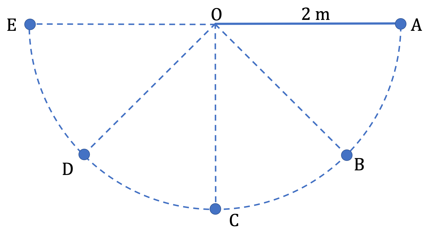
A pendulum swings back and forth. In one of those swings, the pendulum bob goes from A to E shown in the Figure. The speed and magnitude of tangential acceleration at the points marked on the figure are
\begin{align*}
\amp v_A = 0, \ \ \ |a_\theta|_A = 9.81\,\text{m/s}^2\\
\amp v_B = 5.3\,\text{ m/s}, \ \ \ |a_\theta|_B = 7\,\text{m/s}^2\\
\amp v_C = 6.3\,\text{ m/s}, \ \ \ |a_\theta|_C = 0\\
\amp v_D = 5.3\,\text{ m/s}, \ \ \ |a_\theta|_D= 7\,\text{m/s}^2\\
\amp v_E = 0, \ \ \ |a_\theta|_E = 9.81\,\text{m/s}^2
\end{align*}
Find magnitude and direction of the net acceleration at these instants. Note that direction of the swing is important here.
Answer.
(A) \(\vec a_A = -9.81\, \hat j,\text{,}\) (B) \(-\dfrac{21}{\sqrt{2}} \, \hat i + \dfrac{7}{\sqrt{2}} \, \hat j. ,\) (C) \(19.8\text{ m/s}^2\, \hat j,\) (D) \(\dfrac{21}{\sqrt{2}} \, \hat i + \dfrac{7}{\sqrt{2}} \, \hat j,\) (E) \(-9.81\text{ m/s}^2\, \hat j \text{.}\)
Solution.
We need to add the centripetal and tangential accelerations vectorially. Let’s work out thee magnitude and directions of these at eqch instant first. For direction’s sake, let \(x\) axis be pointed to the right and \(y\) pointed Up, and use the unit vectors \(\hat i\) and \(\hat j\text{.}\) You could also do these calculations by keeping track of \(x \) and \(y \) components.
A.
The centripetal and tangential acceleration vectors are:
\begin{align*}
\amp a_c = 0\ \ (\text{since } v = 0.)\\
\amp a_\theta = -9.81\, \hat j.
\end{align*}
Adding then, we get the net acceleration at A to be
\begin{equation*}
\vec a_A = -9.81\, \hat j.
\end{equation*}
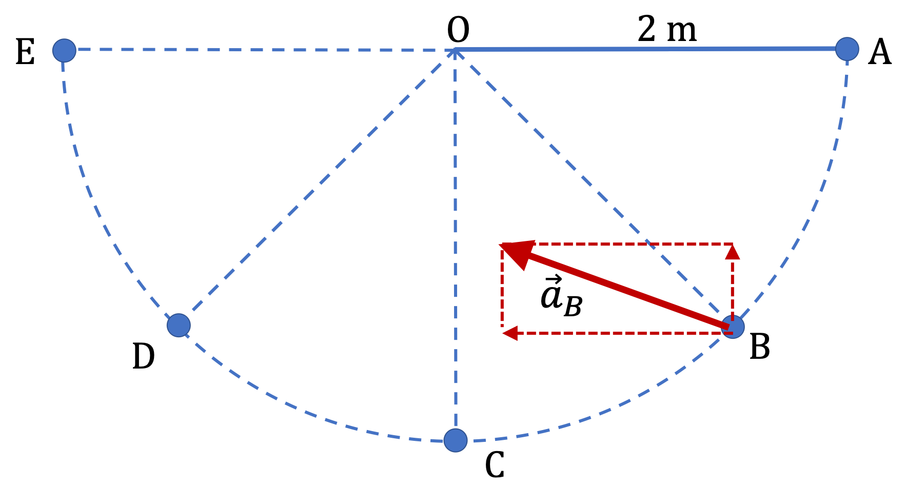
B.
The magnitude of the centripetal acceleration is
\begin{equation*}
a_c = \dfrac{v^2}{R} = \dfrac{5.3^2}{2} = 14.0\text{ m/s}^2.
\end{equation*}
The direction is in the second quadrant in the following unit vector direction.
\begin{equation*}
\hat u_c = -\cos\, 45^{\circ}\, \hat i + \sin\, 45^{\circ}\, \hat j = \dfrac{-\hat i + \hat j}{\sqrt{2}}
\end{equation*}
Similarly, the tangential direction in pointed in the third quadrant.
\begin{equation*}
\hat u_\theta = -\cos\, 45^{\circ}\, \hat i - \sin\, 45^{\circ}\, \hat j = \dfrac{-\hat i - \hat j}{\sqrt{2}}
\end{equation*}
Therefore, the centripetal and tangential accelerations vectors in the component for are:
\begin{align*}
\amp a_c = \dfrac{14.0}{\sqrt{2}} \left( -\hat i + \hat j\right)\\
\amp a_\theta = \dfrac{7}{\sqrt{2}}\left( -\hat i - \hat j\right).
\end{align*}
Adding then, we get the net acceleration at A to be
\begin{equation*}
\vec a_B= -\dfrac{21}{\sqrt{2}} \, \hat i + \dfrac{7}{\sqrt{2}} \, \hat j.
\end{equation*}
That is the acceleration has the magnitude
\begin{equation*}
\sqrt{ \dfrac{21^2}{2} + \dfrac{7^2}{2} } \text{ m/s}^2 = 15.65\,\text{m/s}^2.
\end{equation*}
The direction of acceleration is shown in the figure.
C.
The tangential acceleration here is zero, so the net acceleration is just the centripetal acceleration, which is directed vertically up. Therefore,
\begin{equation*}
\vec a_C = \dfrac{v^2}{R}\, \hat j = 19.8\, \hat j.
\end{equation*}
That is, the magnitude is \(19.8\text{ m/s}^2\text{.}\)
D.
Now, compared to ppoint B, the pendulum bob is slowing. Therefore, tangential acceleration is pointed in the fourth quadrant and the centripetal acceleration, being radial, is pointed in the first quadrant. Draw figures to convince youerself. This will mean that we will have net acceleration towards positive \(x \) direction and same magnitude as in B.
\begin{equation*}
\vec a_D = \dfrac{21}{\sqrt{2}} \, \hat i + \dfrac{7}{\sqrt{2}} \, \hat j.
\end{equation*}
E.
The situation here is same as A since centripetal acceleration is zero and tangential is pointed in the vertically down direction.
\begin{equation*}
\vec a_E = -9.81\text{ m/s}^2\, \hat j.
\end{equation*}


