Section 30.2 Gauss's Law
In Checkpoint 30.1.5, we found that electric flux through a spherical surface around a charge \(q\) to be
It may not surprise you that if you try to find flux through another spherical surface of different radius, you would get the same answer. What is really stunning is that electric flux through any surface enclosing the charge would give the same flux!

Subsection 30.2.1 Statement of Gauss's Law
Gauss's law generalizes the result obtained above to the case of any number of charges and any location of the charges in the space inside the closed surface. According to Gauss's law, the flux of electric field \(\vec E\) through any closed surface is equal to the net charge enclosed \(q_\text{enc}\) divided by the permittivity of free space \(\epsilon_0\text{.}\)
The enclosing surface is arbitrary except that it must be a closed surface. The surface used for this purpose is also called a Gaussian Surface.
\(q_\text{enc}\) is the sum total of all charges inside the space enclosed by the Gaussian surface, using positive number for positive charges and negative number for negative charges. It's important to note that charges outside the closed surface do not contribute! If charges are discrete point charges, then we just sum over them, and if they are described by a continuous charge distribution, then we might need to integrate to find the total enclosed charge.
Subsection 30.2.2 (Calculus) Statement of Gauss's Law
We can replace \(\Phi_{\text{through enclosing surface}}\) in Eq. (30.2.1) by the general definition of electric field flux given in Eq. (30.1.4) in Section 30.1. Let us denote the closed surface by \(\text{S}\) and show by a circle on the integral sign that the surface is a closed surface.
where \(q_\text{enc}\) will be the net charge enclosed within the closed Gaussian surface. We can also replace the enclosed charges on the right side by a sum of discrete charges and an integral over continous charges. We need to restrict them to the volume of space enclosed by \(\text{S}\text{.}\) Thus, we can write a more expnaded view.
We can, of course, think of discrete charges as distributed in a tiny volume and assign it a charge density. Therefore, we should actually drop the \(q_i\) part and absorb that in \(\rho\text{.}\) This gives us the most general way of writing Gauss's law.
Subsection 30.2.3 (Calculus) Divergence of Electric Field
Applying Eq. (30.2.4) for infinitesimal volumes around any arbitray point in space and dividing by the volume of that space gives us an alternate way of looking at Gauss's law.
The left side of this equation is the definiing equation for divegence of electric field, written as \(\vec \nabla \cdot \vec E\text{.}\) The divergence at a point tells us how electric field lines spread out from that point. Therefore,
If you work out the divergence of electric field of a point charge, you will find that it is zero everywhere except at the point where the charge is located.
Checkpoint 30.2.2. Using Gauss's Law To Find Electric Flux Through Closed Surfaces From Charges.
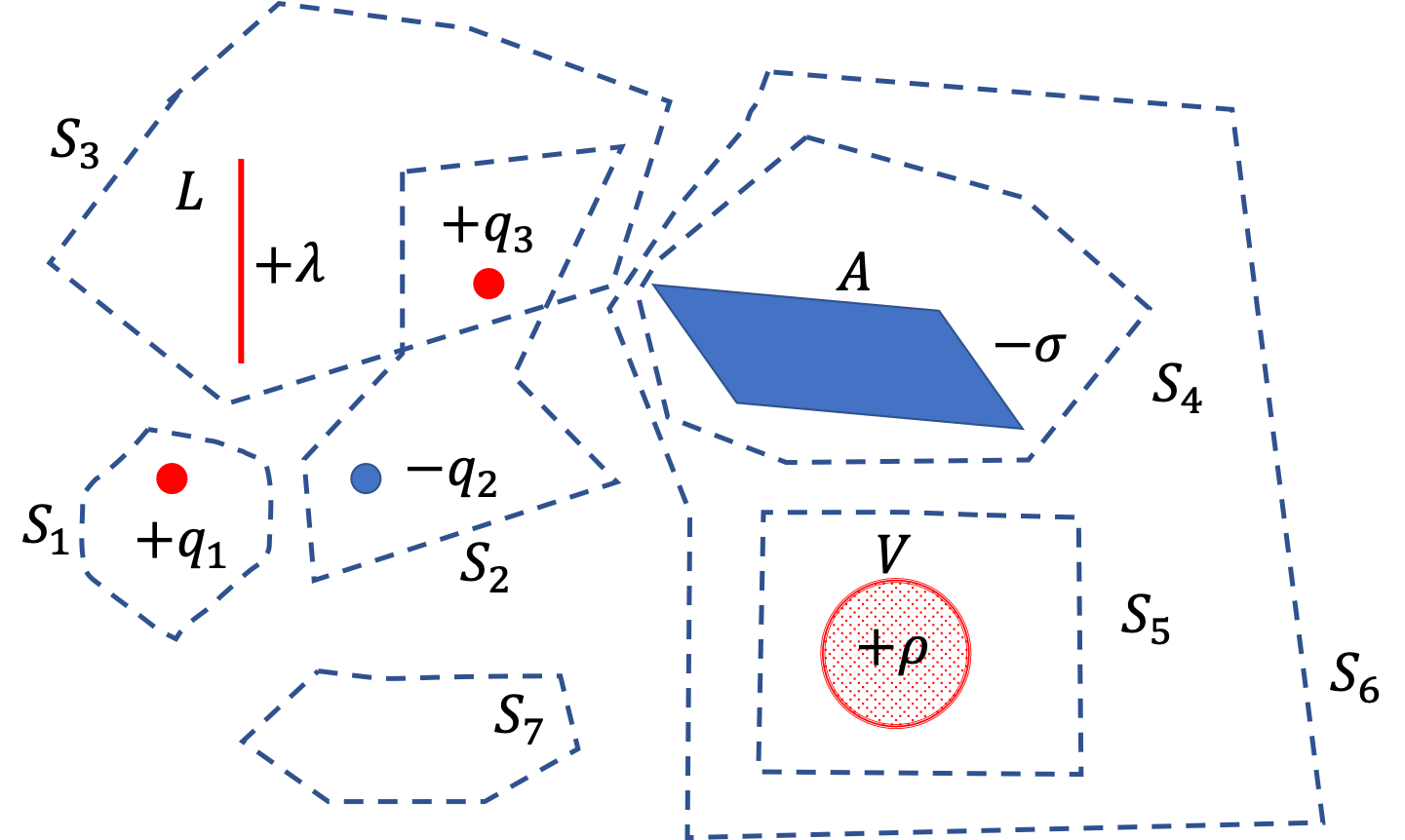
Figure below shows a region of space with three point charges and three uniform charge distribution, one a line charge, another a surface charge distribution, and a volume charge distribution. Find electric flux through each of the seven closed surface shown as dashed line.

Use Gauss's Law.
(1) \(\dfrac{q_1}{\epsilon_0}\text{,}\) (2) \(\dfrac{-q_2+q_3}{\epsilon_0} \text{,}\) (3) \(\dfrac{q_3 + \lambda L}{\epsilon_0}\text{,}\) (4) \(\dfrac{-\sigma\, A}{\epsilon_0}\text{,}\) (5) \(\dfrac{\rho\, V}{\epsilon_0}\text{,}\) (6) \(\dfrac{(-\sigma\, A + \rho\, V)}{\epsilon_0} \text{,}\) (7) \(0\text{.}\)
In each case, we just need to find how much charge there is inside the enclosing surface.
Note the answer for \(\Phi_{S_7}\) - it is zero since there is no charge inside the surface.
Subsection 30.2.4 Applying Gauss's Law to Find Electric Field
Gauss's law is very helpful in determining formulas for magnitude of electric field even though the law is about the electric flux and not directly about the electric field as we will see in examples below. The application hinges on recognizing and applying symmetry in physical situations.
Basically, there are only three types of problems that have the requisite symmetry so that Gauss's law can be fruitfully used to deduce the electric field.
- A charge distribution with a spherical symmetry
- A charge distribution with a cylindrical symmetry
- A charge distribution with a planar symmetry
General Approach:
In each case, based on the symmetry of the charge distribution, we can guess two important aspects of the electric field by that type of symmtery:
- Direction of \(\vec E\text{.}\)
- Functional form of the magnitude, \(E\text{.}\)
Armed with this knowledge, it is possible to find a Gaussian surface which will make flux equal to either zero or a product of \(E\) and some area \(A\text{.}\)
By using the charge distribution, we find the charge that's inside the Gaussian surface we choose. This will give \(q_\text{enc}\text{.}\) Now, we put the expression for flux and \(q_\text{enc}\) in Gauss's law and solve for the magnitude of electric field \(E\text{.}\)
Mathematical details differ considerably in the three types of symmetries. Therefore, I will present each in a separate section.