
Section 4.8 Variable Acceleration

Predictions of velocity and position become more difficult mathematically when acceleration changes with time. You will see that acceleration can change abruptly by simple stopping a force or suddenly turning on a force or channging direction of a force on the body. For instance, when a ball hits the floor, force immediately changes from simple gravity to a combination of gravity and force from the floor. In this case, acceleration which has a value of \(g\) an instant before the touch but it changes to something else right after the ball comes in contact with the ball.

For simplicity, we will first consider motion is one-dimensional on \(x\)-axis so that we have only \(a_x\) nonzero. Since an arbitrarily varying function can always be discretized as constant segments, we can deal with a varying \(a_x\) as a problem of infintely many constant-\(a_x\) problems. In this way, we can build full solution from constant-acceleration formulas applied to each infintesimal time-segments. Let us first consider how to handle a problem that has only two acceleration values.

Subsection 4.8.1 Position and Velocity in a Two-Acceleration Problems

Figure 4.8.1 shows acceleration in a one-dimensional situation along \(x\)-axis that has two values of acceleration. Suppose \(v_{ix}=v_0\) and \(x_i=0\) at \(t=0\text{.}\) We wish to know \(v_x\) and \(x\) at \(t=t_2\text{.}\)

We first work out \(v_x\) and \(x\) at \(t=t_1\text{.}\) Let us denote them by \(v_1\) and \(x_1\text{.}\)

\begin{equation*} v_1 = v_0 + a_1 t_1;\ \ x_1 = v_0t_1 + \frac{1}{2}a_1t_1^2. \end{equation*}

Figure 4.8.1.

Now, we use these values as initial values for the second segment to obtian \(v_2\) and \(x_2\) at \(t=t_2\) using the acceleration of the second segment. Note the time during this segment is not \(t_2\) but \(t_2-t_1\text{.}\)

\begin{align*} v_2 \amp = v_1 + a_2 (t_2-t_1) = v_0 + a_1 t_1 + a_2 (t_2-t_1)\\ x_2 \amp = x_1 + v_1(t_2-t_1) + \frac{1}{2}a_2 (t_2-t_1)^2 \\ \amp = v_0t_1 + \frac{1}{2}a_1t_1^2 + ( v_0 + a_1 t_1 )(t_2-t_1) + \frac{1}{2}a_2 (t_2-t_1)^2 \end{align*}

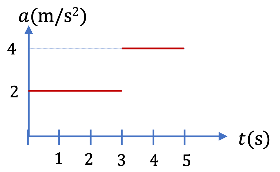
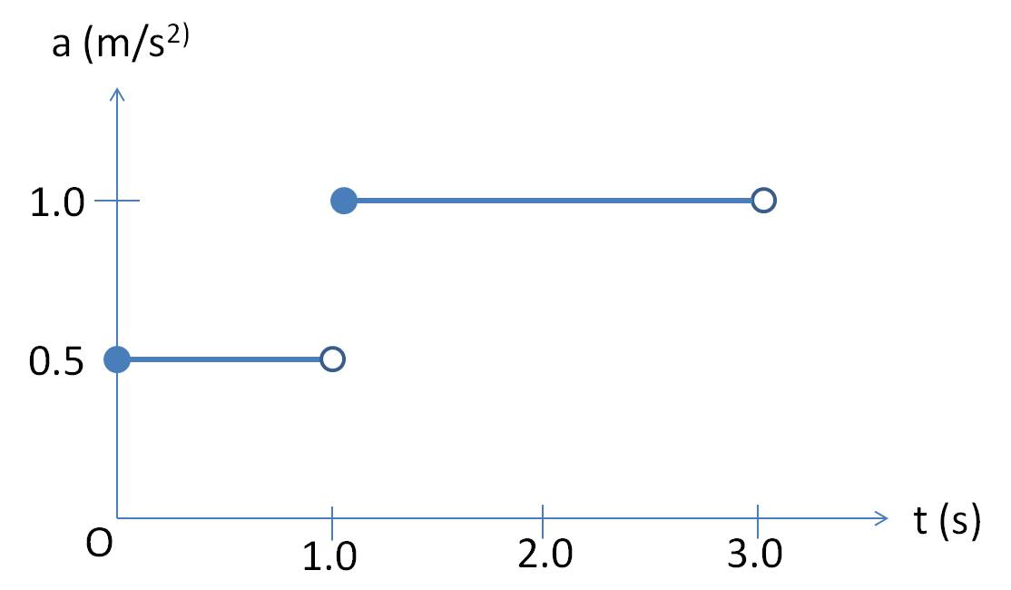
A train starts out at rest and moves in a straight line. The acceleration of the train changes with time, with magnitude \(0.5 \text{ m/s}^2\) between \(t = 0\) and \(t = 1 \text{ sec}\text{,}\) and then with magnitude \(1 \text{ m/s}^2\) between \(t = 1 \text{ sec}\) and \(t =3\ \text{sec}\) as shown in Figure 4.8.3. Find the position and the velocity of the train at \(t = 3 \text{ sec}\text{.}\)

Figure 4.8.3. Figure for Checkpoint 4.8.2.
Hint

Work with one acceleration at a time.

Answer

\(2.5\text{ m/s}\)

Solution

As discussed above, we work out each constant acceleration segment one after the other.

Interval \(t = 0\) to \(t =1 \text{ sec}\text{:}\)

Let's list the information about this interval as follows.

\begin{align*} \amp x_i = 0\ \text{(setting the initial position at the origin);}\\ \amp v_{ix} = 0\ \text{ (initially at rest);}\\ \amp a_x = 0.5 \text{ m/s}^2\ \text{ (constant -acceleration during this interval);}\\ \amp \text{Set t = 0 at the beginning of the interval so that we can use the standard formulas.} \\ \amp t = 1 \text{ s} \ \text{ (duration of this interval);} \end{align*}

With this information, we need to find \(x\) and \(v\text{,}\) the position and velocity at the end of interval.

\begin{align*} \amp v_x = v_{ix} + a_x t = 0 + 0.5\times 1 = 0.5 \text{ m/s};\\ \amp x = x_i + v_{ix} t + \frac{1}{2}a_xt^2 \\ \amp = 0 + 0 + \frac{1}{2}\times 0.5\times 1^2 = 0.25 \text{ m}. \end{align*}

Interval \(t = 1 \text{ sec}\) to \(t =3 \text{ sec}\text{:}\)

Using the information at the end of the previous segment of time, we now know the following information for this interval.

\(x_i = 0.25 \text{ m}\) since initial \(x\)-position here is the final \(x\)-position at the end of the previous interval.

\(v_{ix} = 0.5 \text{ m/s}\) since initial \(x\)-velocity here is the final \(x\)-velocity at the end of the previous interval.

\(a_x = 1.0 \text{ m/s}^2\) since constant \(x\)-acceleration during this interval.

\(t = 2 \text{ s}\) duration of this interval is from \(t= 1\text{ s}\) to \(t = 3 \text{ s}\) or \((3\text{ s}-1\text{ s}=2\text{ s})\text{.}\)

With this information, we need to find \(x\) and \(v_x\text{,}\) the \(x\)-position and \(x\)-velocity at the end of interval.

\begin{align*} \amp v_x = v_{ix} + a t = 0.5 + 1\times 2 = 2.5 \text{ m/s};\\ \amp x = x_i + v_{ix} t + \frac{1}{2}a_xt^2 \\ \amp = 0 + 0.5\times 2 + \frac{1}{2}\times 1.0\times 2^2 = 3.0 \text{ m}. \end{align*}

Therefore, the train is at \(3.0 \text{ m}\) from where it was at \(t=0\) and it is moving at \(2.5\text{ m/s}\) at \(t=3.0 \text{ s}\) mark.

A particle starts out at rest at \(t=0\) and accelerates in a straight line with an acceleration of \(2 \text{ m/s}^2\) from \(t = 0\) to \(t = 3\text{ sec}\text{,}\) and then with an acceleration of \(4\ \text{m/s}^2\) pointed in the same direction from \(t = 3\text{ sec}\) to \(t =5\text{ sec}\text{.}\)

(a) Find the position and the velocity of the particle at \(t = 3\) sec.

(b) Find the position and the velocity of the particle at \(t = 5\) sec.

Hint

Work on each segment as if that was the only segment

Answer

(a) \(9\text{ m},\ 6\text{ m/s}\)m (b) \(29\text{ m},\ 14\text{ m/s}\text{.}\)

Solution

(a) Working between \(t=0\) and \(t=3\text{ sec}\) we get

\begin{align*} v_f \amp = v_i + a t = 0 +2\text{ m/s}^2\times 3\text{ s} = 6\text{ m/s}. \\ x_f \amp = x_i + \dfrac{v_i + v_f}{2}\, t = 0 +3\text{ m/s}\times 3\text{ s} = 9\text{ m}. \end{align*}

(b) When, we work between \(t=3\text{ sec}\) and \(t=5\text{ sec}\text{,}\) the initial condition is same as final condition in the last step. Therefore we jnow have

\begin{equation*} x_i = 9\text{ m},\ \ v_i = 6\text{ m/s}. \end{equation*}

With \(a=4\text{ m/s}^2\text{,}\) we get

\begin{align*} v_f \amp = v_i + a t = 6\text{ m/s} +4\text{ m/s}^2\times 2\text{ s} = 14\text{ m/s}. \\ x_f \amp = x_i + \dfrac{v_i + v_f}{2}\, t = 9\text{ m} +\dfrac{6\text{ m/s} + 14\text{ m/s}}{2}\times 2\text{ s} = 29\text{ m}. \end{align*}

At \(t=0\) a particle located at origin has a velocity of \(20\) m/s in the direction of the positive \(x\)-axis, and accelerates on the \(x\)-axis as shown in the figure. The \(y\) and \(z\)-components of the acceleration are zero.

(a) Find the position and the velocity of the particle at \(t = 2\) sec.

(b) Find the position and the velocity of the particle at \(t = 5\) sec.

Hint

Work on each segment as if that was the only segment

Answer

(a) \(34\text{ m},\ 14\text{ m/s}\)m (b) \(94\text{ m},\ 26\text{ m/s}\text{.}\)

Solution

(a) Working between \(t=0\) and \(t=2\text{ sec}\) we have

\begin{equation*} x_i=0,\ v_i=20\text{ m/s},\ a = -3\text{ m/s}^2,\ t = 2\text{ s}. \end{equation*}

Therefore,

\begin{align*} v_f \amp = v_i + a t = 20\text{ m/s} + (-3\text{ m/s}^2)\times 2\text{ s} = 14\text{ m/s}. \\ x_f \amp = x_i + \dfrac{v_i + v_f}{2}\, t = 0 +17\text{ m/s}\times 2\text{ s} = 34\text{ m}. \end{align*}

(b) When, we work between \(t = 2\text{ sec}\) and \(t = 5\text{ sec}\text{,}\) the initial condition is same as final condition in the last step. Therefore we now have

\begin{equation*} x_i = 34\text{ m},\ v_i = 14\text{ m/s},\ a = 4\text{ m/s}^2,\ t = 3\text{ s}. \end{equation*}

Therefore,

\begin{align*} v_f \amp = v_i + a t = 14\text{ m/s} + 4\text{ m/s}^2\times 3\text{ s} = 26\text{ m/s}. \\ x_f \amp = x_i + \dfrac{v_i + v_f}{2}\, t = 34\text{ m} +\dfrac{14\text{ m/s} + 26\text{ m/s}}{2}\times 3\text{ s} = 94\text{ m}. \end{align*}

Suppose you accelerate your car at a constant rate of \(2.0\text{ m/s}^2\) starting from rest for some unspecified time. After that you immediately apply your brake and decelerate at \(5.0\text{ m/s}^2\) and come to a stop. The total distance covered between start and stop was \(800\text{ m}\text{.}\) (a) Find the peak velocity. (b) Find the total time it was in the accelerating phase. (c) Find the total time it was in the decelerating phase.

Solution

No solution provided.

Subsection 4.8.2 (Calculus) Arbitrarily Varying Acceleration

Although most of our examples in this book will have constant-acceleration segments, it is worthwhile to look at a case of arbitrarily varying acceleration as an important extension of the multi-step method presented above. We will assume only \(a_x\) is nonzero, and, for brevity, use \(a\) for \(a_x\text{.}\)

The basic idea for handling an arbitrarily varying acceleration is to replace the original acceleration by an approximation obtained by dividing up the time interval of interest into smaller time intervals. If time segments are small enough, we can approximate the original arbitrarily varying acceleration by a step-wise varying acceleration, where each step is an average acceleration in the corresponding time segment. This is often called discretizing acceleration.

Clearly the original situation of a continuously varying acceleration is not the same as its replacement by constant acceleration steps. However, Isaac Newton showed that if intervals were allowed to be arbitrarily small, then the predictions of final position and velocity, based on step-wise approximate acceleration, can be made arbitrarily close to the exact answer without the approximation (see Figure 4.8.7.)

Figure 4.8.7. A varying acceleration (a) and successive approximate constant acceleration steps of different step sizes (b, c and d). In (b) the variable acceleration is replaced by one constant step with the average acceleration denoted as \(a_1\) in (b). In (c) the variable acceleration is replaced by two segments of constant acceleration steps of \(a_1\) and \(a_2\text{.}\) Similarly, in (d) the variable acceleration is replaced by four steps. The process can be continued ad-infinitum. As you decrease the step size, or equivalently increase the number of steps, the original acceleration is covered more accurately by the approximation.

With this approximation scheme, it is possible to find changes in velocity over the entire finite interval, from \(t = 0\) to \(t = T\text{,}\) not just over one of the small steps.

Let us divide the interval \([0,T]\) into \(N\) equal intervals: \([0, \Delta t)\text{,}\) \([\Delta t, 2\Delta t )\text{,}\) \([2\Delta t, 3\Delta t)\text{,}\) \(\cdots\) \([(N-1)\Delta t, N\Delta t]\text{.}\) The time \(N\Delta t\) is equal to the total time \(T\) of all the intervals added. Let acceleration in thes subintervals be \(a_1\text{,}\) \(a_2\text{,}\) \(a_3\text{,}\) \(\cdots\) , \(a_N\text{,}\) respectively. Let \(v_1\text{,}\) \(v_2\text{,}\) \(v_3\text{,}\) \(\cdots\) , \(v_N\) be velocities at the end of the corresponding intervals. Of course \(v_N\) is same as \(v(T)\) or simply \(v\) at the end of the final time. Now, we show that our procedure leads us to the prediction of the final velocity from the initial velocity \(v_0\text{,}\) the velocity at time \(t=0\text{.}\)

Interval Velocity at the end of the interval
\(0 \text{ to } \Delta t \) \(v_1 = v_0 + a_1 \Delta t\)
\(\Delta t \text{ to } 2\Delta t \) \(v_2 = v_1 + a_2 \Delta t\)
\(2\Delta t \text{ to } 3\Delta t \) \(v_3 = v_2 + a_3 \Delta t\)
\(3\Delta t \text{ to } 4\Delta t \) \(v_4 = v_3 + a_4 \Delta t\)
\(\vdots \) \(\vdots \)
\((N-2)\Delta t \text{ to } (N-1)\Delta t \) \(v_{N-1} = v_{N-2} + a_{N-1} \Delta t\)
\((N-1)\Delta t \text{ to } N\Delta t \) \(v_{N} = v_{N-1} + a_{N} \Delta t\)
\(0 \text{ to } N\Delta t \) \(v_{N} = v_{0} + \sum_{i=1}^{N}a_{i} \Delta t\)

Summing the velocity change equation in each interval gives us the following equation for the change in velocity from \(v_0\) to \(v\) over the entire time \([0,T]\text{.}\)

\begin{equation} v = v_0 + \sum_{i=1}^{N} a_i \Delta t. \label{eq-var-acc-vel-1}\tag{4.8.1} \end{equation}

The approximation becomes better as \(\Delta t\) is made smaller. We denote the limit of the summation as \(\Delta t\) approaches zero by another symbol, called the definite integral of \(a(t)\) from \(t = 0\) to \(t = T\text{.}\)

\begin{equation} v - v_0 = \int_{0}^{T} a(t) dt, \ or, (\text{Area under the curve of }a \text{ vs } t).\label{eq-var-acc-vel-2}\tag{4.8.2} \end{equation}

For an arbitrary interval t = t1 to t= t2, the integration will be done accordingly.

\begin{equation*} v_2 - v_1 = \int_{t_1}^{t_2} a(t) dt. \end{equation*}

Similar arguments will lead you to analogous relation between change in position and velocity as we found between change in velocity and acceleration. We give the result for future reference and leave the derivation as an exercise for the student. Denoting average velocities in segments \(1, 2, 3, \cdots, N\) as \(\bar v_1, \bar v_2, \bar v_3, \cdots, \bar v_N\) we will obtain the following change in position \(x-x_0\) for the total time \(T=N\Delta t\text{.}\)

\begin{equation*} x - x_0 = \sum_{i=1}^N \bar v_i\Delta t \Longrightarrow \int_0^T v(t) dt,\ or, (\text{Area under the curve of }v \text{ vs } t). \end{equation*}

For an arbitrary interval t = t1 to t= t2, the integration will be done accordingly.

\begin{equation*} x_2 - x_1 = \int_{t_1}^{t_2} v(t) dt. \end{equation*}

The \(x\)-component of the acceleration of a particle changes according to the following analytic expression, \(a_x(t) = 4+t^2/2\text{,}\) where \(t\) is in sec and the acceleration in \(\text{m/s}^2\text{.}\) Find the \(x\)-components of the velocity and position vectors. Use \(v_0\) and \(x_i\) for initial velocity and initial position respectively.

Hint

\(v_x(t) - v_x(0) = \int_0^t\, a_x dt\text{.}\)

Answer

(a) \(x = x_i + v_0 t + 2 t^2 + \dfrac{1}{24} t^4\text{,}\) (b) \(v = v_0 + 4 t + \dfrac{1}{6} t^3 \text{.}\)

Solution

Integrating \(a_x(t)\) will give \(v_x(t) - v_0\) and integrating \(v_x(t)\) will give \(x(t)-x_i\text{.}\)

\begin{align*} v_x(t) \amp = v_x(0) + \int_0^t\, a_x dt \\ \amp = v_0 + \int_0^t\,\left( 4+t^2/2 \right) dt \\ \amp = v_0 + 4 t + \dfrac{1}{6} t^3. \\ x(t) \amp = x(0) + \int_0^t\, v_x(t) dt \\ \amp = x_i + \int_0^t\, \left(v_0 + 4 t + \dfrac{1}{6} t^3 \right) dt \\ \amp = x_i + v_0 t + 2 t^2 + \dfrac{1}{24} t^4. \end{align*}