Quantum Tunneling

Section 54.7 Quantum Tunneling

Suppose you are in some playground fenced with a 10-foot fence and someone told you that you can just pass through the fence without having enough energy to climb over the fence, you would think that is not possible. But, Shcrödinger equation predicts that a quantum particle can get through a finite barrier even when it does not have enough energy. This phenomenon is called quantum tunneling. The tunneling phenomenon is observed in a variety of quantum systems and considered one of the fundamental difference between quantum mechanics and classical mechanics.

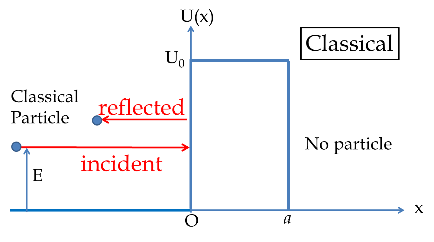
Figure 54.7.1 illustrates the difference between classical and quantum behaviors of a particle incident on a finite barrier with energy less than the energy of the barrier. A classical particle will not be able to penetrate the barrier while a quantum particle will have a finite probability of being found on the other side of the barrier.

Figure 54.7.1. The tunneling of a quantum particle through a finite barrier. Classically, the particle will be reflected back and would not be found on the other side of the barrier, but quantum mechanically, there is a probability that the particle will be found on the other side of the barrier!

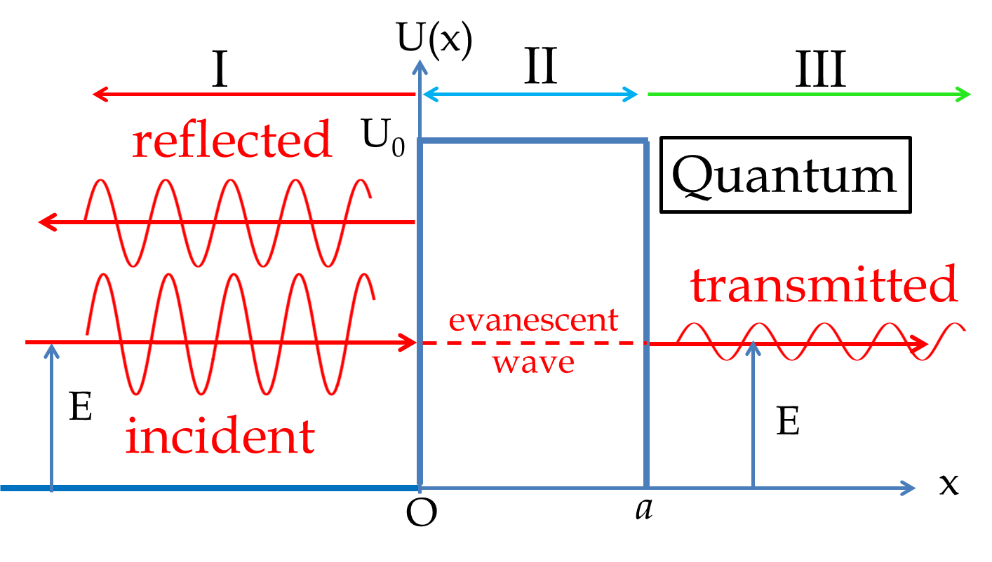
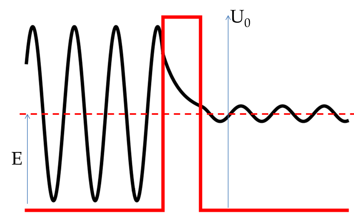
Here, we will work out a simple problem of tunneling through a finite barrier. Consider an incoming wave $\psi_{in}$ of energy $E$ traveling from $x=-\infty$ towards the positive $x$-axis. The wave encounters a barrier of potential energy of the barrier $U_0$ which is greater than the energy $E$ of the particle. The barrier is of constant height until $x=a$ and then let the potential energy be back to zero again. We want to know if there is any probability that the particle will be found on the other side of the barrier, i.e., in region $x>a\text{.}$

As in the last problem it is convenient for calculation to introduce the following constants.

\begin{equation} k = \dfrac{\sqrt{2mE}}{\hbar},\quad \alpha = \dfrac{\sqrt{2m(U_0-E)}}{\hbar},\quad \omega = \dfrac{E}{\hbar}.\tag{54.7.1} \end{equation}

We will look at a stationary state of a definite energy $E\text{.}$ Then the wave function will be taken to have the following time behavior.

\begin{equation} \psi(x,t) = \psi_E(x) e^{-i\omega t},\tag{54.7.2} \end{equation}

where $\psi_E(x)$ is the time-independent wave function which will depend on the region of the $x$-axis. The problem has three regions, labeled I, II, and III in the figure. In regions I and III, the energy is greater than the potential energy in these region and the Schr\"odinger equation takes the following form.

\begin{equation} \textrm{Regions I and III:}\quad\dfrac{\partial ^2 \psi_E}{\partial x^2} = -k^2 \psi_E.\tag{54.7.3} \end{equation}

The general solution of this equation in exponential complex notation is

\begin{equation} \psi_E(x) = A_{+} e^{ikx} + A_{-} e^{-ikx},\tag{54.7.4} \end{equation}

where $A_{+}$ and $A_{-}$ are the amplitudes of waves moving towards the positive and negative $x$-axis, respectively. We are interested in wave coming from the negative $x$-axis and making its way towards the positive $x$-axis in region III. Therefore, in region I the wave will be a superposition of an incoming wave traveling towards the positive $x$-axis and a reflected wave traveling towards the negative $x$-axis, and in region III, the wave will be just a wave traveling towards the positive $x$-axis. Let us denote the waves in the three regions by subscripts I, II and III to $\psi\text{.}$

\begin{equation} \begin{array}{l} \psi_I = \psi_{in} + \psi_{re} = A e^{ikx - i\omega t} + B e^{-ikx - i\omega t}.\\ \psi_{III} = \psi_{tr} = F e^{ikx - i\omega t}. \end{array} \label{eq-tunneling-wave-functions-region-1}\tag{54.7.5} \end{equation}

In region II, the energy is less than the potential energy. That means the kinetic energy will be negative. The time-independent Schr\"odinger equation for region II in the new variables defined above is

\begin{equation} \textrm{Regions II:}\quad\dfrac{\partial ^2 \psi_E}{\partial x^2} = +\alpha^2 \psi_E.\tag{54.7.6} \end{equation}

Due to the plus ($+$) on the right side, the solutions of this equation ar ereal exponentials rather than complex exponentials. The wave function is not a traveling wave in this region. The wave function is called evanescent waves.

\begin{equation} \psi_{II}(x) = C e^{\alpha x } + D e^{-\alpha x}\tag{54.7.7} \end{equation}

Summarizing, the solutions of the full Schr\"odinger equation in the three regions for a wave that is coming from $x=-\infty$ are

\begin{equation} \begin{array}{ll} \psi_I = A e^{ikx - i\omega t} + B e^{-ikx - i\omega t} \amp \quad x\lt 0\\ \psi_{II} = C e^{\alpha x - i\omega t} + D e^{-\alpha x - i\omega t} \amp \quad 0\le x \le a\\ \psi_{III} = F e^{ikx - i\omega t} \amp \quad x>a \end{array}\label{eq-tunneling-wave-functions}\tag{54.7.8} \end{equation}

The flux of particles that get transmitted per unit flux of particles that came from $x=-\infty$ to the barrier is

\begin{equation} |j_{tr}|/|j_{in}| = |F|^2/|A|^2,\tag{54.7.9} \end{equation}

where $j_{in}$ is the probability current of the wave $\psi_{in} = A e^{ikx - i\omega t}$ in the region $x \lt 0$ and the $j_{tr}$ is the probability current of the wave $\psi_{tr} = A e^{ikx - i\omega t}$ in the region $x>a\text{.}$ Therefore, the probability of transmission will be

\begin{equation} P(\textrm{of tunneling}) = \left|\dfrac{F}{A}\right|^2.\label{eq-tunneling-prob-1}\tag{54.7.10} \end{equation}

We use the boundary conditions at $x=0$ and $x=a$ to determine the expression for the coefficients in the wave functions in Eq. (54.7.8). The boundary conditions come from the continuity of the wave function and its space derivative at finite potential steps. Here, we will have the following four conditions.

\begin{align*} \amp \psi_I(0,t) = \psi_{II}(0,t), \amp \amp \left|\dfrac{\partial \psi_I}{\partial x}\right|_{x=0} = \left|\dfrac{\partial \psi_{II}}{\partial x}\right|_{x=0}.\\ \amp \psi_{II}(a,t) = \psi_{III}(a,t), \amp \amp \left|\dfrac{\partial \psi_{II}}{\partial x}\right|_{x=a} = \left|\dfrac{\partial \psi_{III}}{\partial x}\right|_{x=a}. \end{align*}

These conditions give the following relations.

\begin{align*} \amp A + B = C+D, \amp \amp k(A - B) = \alpha (C - D).\\ \amp C e^{\alpha a} + D e^{-\alpha a} = F e^{ika}, \amp \amp \alpha\left(C e^{\alpha a} - D e^{-\alpha a} \right) = ik F e^{ika}. \end{align*}

The calculation of $F/A$ requires eliminating $B\text{,}$ $C\text{,}$ and $D$ from these four equations. The calculation is tedious and the final result complicated. We will not go into the details of the calculation and leave the exercise to a more enterprising student. After you have calculated, you will find the result shown in Figure 54.7.2. There will be traveling waves on the left and right of the barrier and an evanescent wave within the barrier which seamlessly connects the wave function on the left of the barrier to the wave function on the right.

Figure 54.7.2. The tunneling of a quantum particle through a finite barrier. We find traveling waves on the two sides of the barrier and a non-traveling wave, called evanescent wave inside the barrier.

A complete calculation shows that the probability of tunneling varies with the gap $U_0 - E$ through the parameter $\alpha$ and the width $a$ exponentially. When the tunneling transmission coefficient is much less than 1, then one can show that the transmission coefficient $T$ varies exponentially with the width of the barrier.

\begin{equation} T = |F/A|^2 \sim 16\frac{E}{U_0}\left(1- \frac{E}{U_0} \right)e^{-2\alpha a}.\label{eq-tunneling-prob-3}\tag{54.7.11} \end{equation}

The factors multiplying the exponential can usually be ignored when analyzing tunneling for system of a given energy. Thus,

\begin{equation} \begin{array}{l} 1.\ \textrm{Larger the} \ U_0 - E\ \textrm{gap},\ \textrm{the larger}\ \alpha\ \textrm{the smaller the probability of tunneling} \\ 2.\ \textrm{Wider the barrier, i.e. larger}\ a,\ \textrm{the smaller the probability of tunneling} \end{array}\nonumber\tag{54.7.12} \end{equation}

Subsection 54.7.1 Scanning Tunneling Microscope

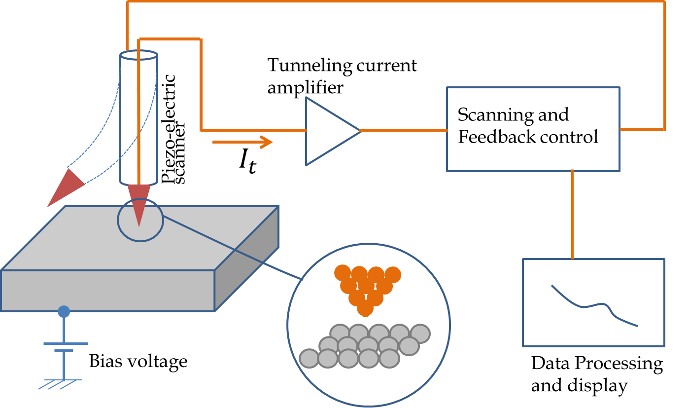
Scanning electron microscope (STM) is an instrument that uses quantum tunneling effect to map a metal surface at the atomic resolution without touching the surface. The STM was invented in early 1980s by Heinrich Rohrer and Gerd Binning at the IBM Research Lab in Zurich, for which they were awarded Nobel prize in physics in 1986.

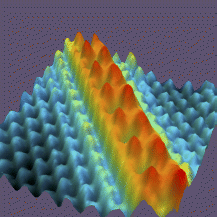
A schematic picture of a STM apparatus is shown in Figure 54.7.3. In an STM machine a sample is approached with a fine tip and a voltage is applied between the sample the tip. If the tip is sufficiently close, i.e. if the distance between the nearest atom of the tip and the sample $a$ is small enough, a current to flow due to tunneling of electrons across the gap.

Figure 54.7.3. Schematics of a scanning tunneling microscope. Electrons jump through the empty space between the tip and the sample, which serves as the tunneling barrier.

The sensitivity of STM

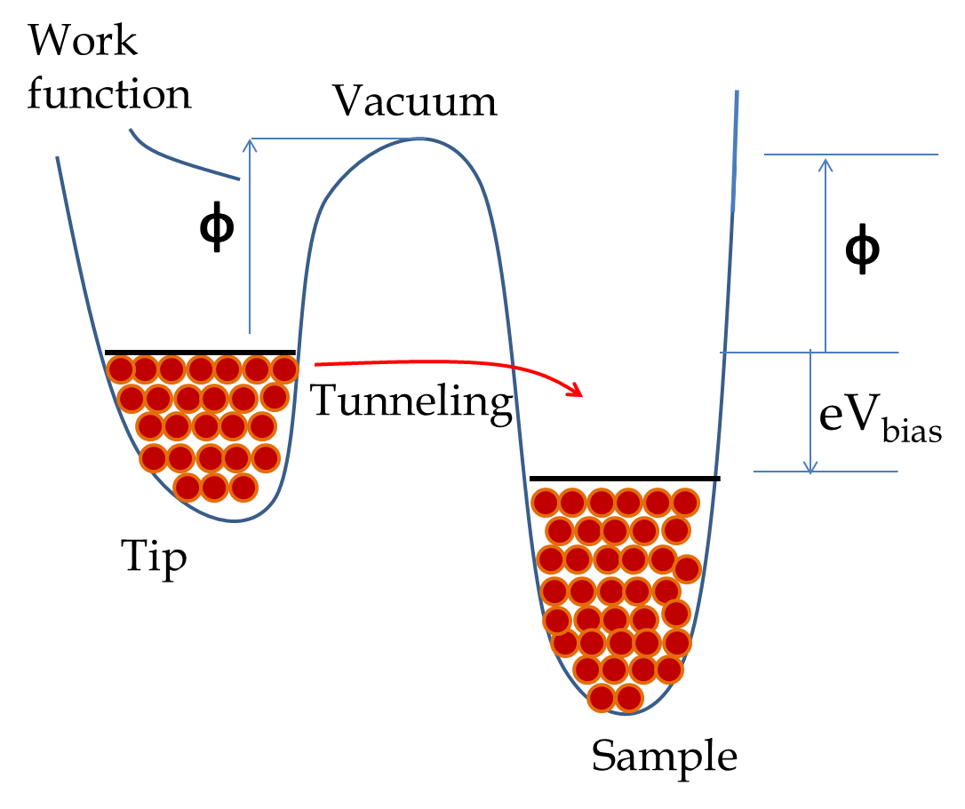
The tunneling current will be proportional to the tunneling probability given by Eq. (54.7.11) with $\alpha$ given by the work function of the metal of the tip or the sample depending upon the way the bias direction. Figure 54.7.4 shows energy diagram for a bias that lower the energy of electron in the sample and the electron flow from the tip to the sample, the electron faces the barrier of the work function of the tip. The tunneling current $I(t)$ drops off exponentially with respect to the distance $a$ between the tip and the surface.

\begin{equation} I = \textrm{constant}\times V_{\textrm{bias}} e^{-2\alpha a}, \label{eq-scan-tunneling-prob-1}\tag{54.7.13} \end{equation}

where $\alpha$ depends on the barrier $\phi$ as

\begin{equation*} \alpha = \dfrac{\sqrt{2 m\phi}}{\hbar} \end{equation*}

Figure 54.7.4. Schematics of energetics of the flow of electron between the tip and the sample.

The bias voltage is usually in the range of 1-2 volts and the work function of most metals is a few electronvolts (eV). For instance, the work function of tungsten and copper, most commonly used metals, are 4.5 eV. For fixed bias and work function, the tunneling current is a very strong function of the separation distance $a\text{.}$ If you increase the separation by $\Delta a\text{,}$ the ratio of the new current to the old current will be

\begin{equation} \dfrac{I(a+\Delta a)}{I(a)} = e^{-2\alpha \Delta a}. \label{eq-scan-tunneling-prob-2}\tag{54.7.14} \end{equation}

Taking the work function $\phi = 4.5 \:\textrm{eV}$ we have

\begin{equation*} \alpha = \dfrac{\sqrt{2 \times 9.1\times 10^{-31}\:\textrm{kg}\times 4.5\times1.6\times 10^{-19} \:\textrm{J}}}{1.055\times 10^{-34}\:\textrm{J.s}} = 1.086\times 10^{-10}\:\textrm{m}^{-1}. \end{equation*}

For a movement of $\Delta = 0.5\:\textrm{nm}\text{,}$ a typical diameter of an atom, we will get the following factor of reduction in the tunneling current.

\begin{align*} \dfrac{I(a+0.5\:\textrm{nm})}{I(a)} \amp = e^{-2\times 1.086\times 10^{-10}\:\textrm{m}^{-1}\times 0.5\times 10^{-9}\:\textrm{m}}\\ \amp = 1.93\times 10^{-5}. \end{align*}

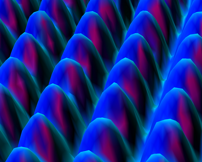
This calculation shows that the current varies over five orders in the course of the movement of one atom. An STM can be operated in a constant-current mode or a constant-height mode. In a constant current mode, the height of the tip is adjusted to maintain the value of tunneling current constant. The adjustments of the height $z$ yield the surface profile in the $xy$-plane as the sample is scanned. In the constant-height mode, the distance between the tip and the sample is kept fixed and current is measured which is then used to deduce the surface profile. The high-resolution surface profiles show vividly the periodicity of crystals and defects on the surface as shown in Figure 54.7.5.

Figure 54.7.5. Examples of STM images. Left image is: Ni crystal surface (Image courtesy of IBM). The right image is: Cesium atoms arranged in a zig-zag on a Ga-As lattice (Image courtesy of NIST).

TODO: \begin{exercise} Electrons of energy 10 eV are incident on a finite barrier of energy 20 eV and width 1 nm. What is the percentage of electrons that will tunnel through the barrier? \end{exercise} \begin{exercise} An electron of energy $E$ is incident on a potential barrier of height $U_0>E$. What will happen to the probability of tunneling if (a) the width of the barrier is doubled, (b) the width of the barrier is halved? \end{exercise} \begin{exercise} The current in the Scanning Tunneling Microscope is proportional to the probability of electrons tunneling between the tip and the surface of the metal. In an experiment the tunneling current increased from $I_0$ to $2I_0$ when the tip is moved from a distance $z$ to $z-\Delta z$ from the sample. Find $\Delta z$ in units of $1/\alpha$, where \[ \alpha = \frac{\sqrt{2m\phi}}{\hbar}, \] where $\phi$ is the work function of the metal. \end{exercise} \begin{exercise} In an unstable nucleus a neutron of energy $E = 1$ MeV is trapped inside a finite potential barrier of height $U_0 = 100$ MeV. Let the width of the nucleus be 3 fm. Estimate the probability that the neutron will tunnel out of the nucleus. \end{exercise} \begin{exercise} The alpha decay of a radioactive nucleus can be modeled as a quantum tunneling effect for alpha particles, which are particles that contain two protons and two neutrons, i.e. the nucleus of the Helium atom. In an unstable nucleus an alpha particle of energy $E = 2$ MeV is trapped by a potential barrier of height $U_0 = 40$ MeV and width 5 fm. Estimate the probability that the alpha particle will tunnel out of the nucleus. \end{exercise}