
Section 45.4 Electromagnetic Waves

One of the early successes of Maxwell's equations was the prediction that light consists of electromagnetic waves. Maxwell came to this conclusion by examining his equations in vacuum. He found that his equations simplify to wave equations for electric and magnetic fields with wave speed given by

\begin{equation*} v_s = \dfrac{1}{\sqrt{\epsilon_0\mu_0}}. \end{equation*}

Let's see what value you would get when you pluch in the values of \(\epsilon_0\) and \(\mu_0\) in SI units.

\begin{align*} v_s \amp = \dfrac{1}{\sqrt{\epsilon_0\mu_0}}\\ \amp = \dfrac{1}{\sqrt{8.852\times 10^{-12}\times 4\pi\times 10^{-7}} }\\ \amp = 3.0\times 10^{8}\text{ m/s}, \end{align*}

which is the value of speed of light, usually denoted by \(c\text{,}\) in vacuum. Maxwell noticed this coincidence and asserted that this mathematical result implied that light is an electromagnetic wave. At that time light was an independent field of study. This conclusion unified the subjects of electricity, magnetism, and optics, and made optics a subfield of electricity and magnetism.

We will see below that electromagnetic wave in vacuum is a transverse wave where electric and magnetic field are perpendicular to each other and to the direction of wave. For instance, if wave is moving in \(x\) direction, then \(\vec E\) and \(\vec B\) will be pointed in directions in \(yz\text{,}\) plane. Furthermore, if \(\vec E\) is pointed towards positive \(y\) axis, then \(\vec B\) will be pointed towards \(z\) axis.

\begin{equation*} \text{Vector product }\vec E \times \vec B \text{ points towards wave flow.} \end{equation*}

Subsection 45.4.1 Hertz's Experiment For Production And Detection Of EM Waves

After Maxwell predicted the existence of the electromagnetic waves in 1873, many scientists tried to produce them in the laboratory. The first person to succeed was the German physicist Heinrich Hertz who produced and detected radio waves in 1888. Hertz's equipment consisted of a radiator and a detector/receiver, a replica of which is shown in Figure 45.4.1.

Figure 45.4.1. A replica of Heinrich Hertz'e apparatus for production and detection of radio waves. Photo courtesy of http://www.sparkmuseum.com/HERTZ.HTM.

The radiator was a pair of one-meter rods with a spark gap in the center and two large spheres at the other ends of the wires to adjust the capacitance for resonance condition. The rods were connected to an induction coil that supplied a high voltage. The receiver was simply a loop of wire with a small gap. When the rods of the radiator setup were given strong enough voltage, a spark was generated across the gap and the current would oscillate back and forth across the gap and along the rods.

The receiver consisted of a loop of wire with a tiny gap. When an electromagnetic waves passes through the area of the loop, the magnetic field in the electromagnet wave would cause the magnetic flux to change which would result in an induced EMF in the wire. The induced EMF caused a spark across the tiny gap in the ring.

Hertz conducted many experiments measuring the wavelength and speed of these waves and showed that they travel at the predicted speed of light. He also showed that the radio waves refracted and reflected similar to light thus lending a strong support to Maxwell's assertion that the light was an electromagnetic wave. When his students asked what use can be made of this discovery, he apparently replied, “It's of no use whatsoever. This is just an experiment that proves Maestro Maxwell was right - we just have these mysterious electromagnetic waves that we cannot see with the naked eye. But they are there.” But, here we are today about 100 years later with our cell phones and WiFi none of which would be possible without Hertz's discoveries. To honor Hertz the unit of frequency Hertz (Hz) is named after Heinrich Hertz. One Hertz equals one cycle per second.

Subsection 45.4.2 Plane Electromagnetic Waves

To arrive at Maxwell's discovery we seek a solution of his equations in region of space that has no currents (\(\vec J = 0\)) or charges (\(\rho = 0\)), so-called empty space or vacuum.

\begin{align} \amp \vec{\nabla}\cdot \vec E = 0 \label{eq-max-empty-1}\tag{45.4.1}\\ \amp \vec{\nabla}\cdot \vec B = 0 \label{eq-max-empty-2}\tag{45.4.2}\\ \amp \vec{\nabla}\times \vec E = -\frac{\partial \vec B}{\partial t} \label{eq-max-empty-3}\tag{45.4.3}\\ \amp \vec{\nabla}\times \vec B =\mu_0\epsilon_0 \frac{\partial \vec E}{\partial t} \label{eq-max-empty-4}\tag{45.4.4} \end{align}

For simplicity we seek EM waves moving in the \(x\) direction and electric and magnetic fields that are independent of \(y\) and \(z\text{.}\) We make a further simplification: let the electric field have only the \(y\)-component everywhere. These choices leave only \(E_y\) and \(\vec B\) to be determined and their dependences are reduced to only two variables \(x\) and \(t\text{.}\)

\begin{equation*} \text{Unknowns:}\ \ E_y(x,t)\ \ \text{and}\ \ \vec B(x,t). \end{equation*}

Writing out the first Maxwell's equation, Eq. (45.4.1) for the empty space explicitly in the Cartesian coordinates we find that it is automatically satisfied by the assumed component and functional dependence of electric field.

\begin{equation*} \vec{\nabla}\cdot\vec E = \frac{\partial E_x}{\partial x} + \frac{\partial E_y}{\partial y} + \frac{\partial E_z}{\partial z} = 0. \end{equation*}

We now look at the components of the third Maxwell's equation, the Faraday law given in Eq. (45.4.3), keeping only the non-zero terms.

\begin{align*} \amp x\text{-component:}\ \ \frac{\partial E_z}{\partial y} - \frac{\partial E_y}{\partial z} = -\frac{\partial B_x}{\partial t} \Longrightarrow \frac{\partial B_x}{\partial t} =0\\ \amp y\text{-component:}\ \ \frac{\partial E_x}{\partial z} - \frac{\partial E_z}{\partial x} = -\frac{\partial B_y}{\partial t} \Longrightarrow \frac{\partial B_y}{\partial t} =0\\ \amp z\text{-component:}\ \ \frac{\partial E_y}{\partial x} - \frac{\partial E_x}{\partial y} = -\frac{\partial B_z}{\partial t} \Longrightarrow \frac{\partial E_y}{\partial x} = -\frac{\partial B_z}{\partial t} \end{align*}

Since the \(x\)- and \(y\)-components of \(\vec B\) are independent of time, they will not be in the wave solution. Therefore, we will set them to zero.

\begin{equation*} B_x = 0;\ \ \ B_y = 0. \end{equation*}

This leaves only \(E_y\) and \(B_z\) non-zero.

\begin{equation*} \text{Unknowns left:}\ \ E_y(x,t)\ \ \text{and}\ \ B_z(x,t). \end{equation*}

Finally, we work out the components of the Ampere-Maxwell's law when \(\vec E\) and \(\vec B\) are independent of \(y\) and \(z\text{.}\)

\begin{align*} \amp x\text{-component:}\ \ \frac{\partial B_z}{\partial y} - \frac{\partial B_y}{\partial z} = \mu_0 \epsilon_0 \frac{\partial E_x}{\partial t} \Longrightarrow 0 =0\nonumber\\ \amp y\text{-component:}\ \ \frac{\partial B_x}{\partial z} - \frac{\partial B_z}{\partial x} = \mu_0 \epsilon_0\frac{\partial E_y}{\partial t} \Longrightarrow \frac{\partial B_z}{\partial x} = - \mu_0 \epsilon_0\frac{\partial E_y}{\partial t}\\ \amp z\text{-component:}\ \ \frac{\partial B_y}{\partial x} - \frac{\partial B_x}{\partial y} = \mu_0 \epsilon_0\ \frac{\partial E_z}{\partial t} \Longrightarrow 0 = 0 \end{align*}

where I have written \(0 = 0\) for the equations that are automatically satisfied. These calculations show that \(E_y\) and \(B_z\) are not independent. They are related by

\begin{align} \amp \frac{\partial E_y}{\partial x} = -\frac{\partial B_z}{\partial t} \label{eq-ey-from-bz-1}\tag{45.4.5}\\ \amp \frac{\partial B_z}{\partial x} = - \mu_0 \epsilon_0\frac{\partial E_y}{\partial t} \label{eq-ey-from-bz-2}\tag{45.4.6} \end{align}

These two equations show that you do not have to solve for both \(E_y\) and \(B_z\text{.}\) If you know one, you can get the other. Therefore, the number of unknowns now becomes one.

\begin{equation*} \text{Unknowns: either}\ E_y \text{ or }\ B_z. \end{equation*}

We can eliminate \(E_y\) or \(B_z\) from Eqs. (45.4.5) and (45.4.6) to obtain separate equations for \(E_y\) and \(B_z\text{,}\) only one of which we need to solve.

\begin{align} \amp \frac{\partial^2 E_y}{\partial x^2} = \mu_0\epsilon_0 \frac{\partial^2 E_y}{\partial t^2}\label{eq-em-wave-eq-e}\tag{45.4.7}\\ \amp \frac{\partial^2 B_z}{\partial x^2} = \mu_0\epsilon_0 \frac{\partial^2 B_z}{\partial t^2} \label{eq-em-wave-eq-b}\tag{45.4.8} \end{align}

Suppose we choose to solve for \(E_y\text{.}\) A simple solution of Eq. (45.4.7) is a traveling wave along the \(x\)-axis with a speed \(v\text{.}\)

\begin{equation} E_y(x,t) = E_0\cos\left[ k(x \pm vt) \right]. \label{eq-soln-ey-wave-0}\tag{45.4.9} \end{equation}

Here the minus sign corresponds to a wave moving in the direction of the positive \(x\)-axis and the plus sign to the wave moving towards the negative \(x\)-axis. This solution must satisfy Eq. (45.4.7). Plugging into Eq. (45.4.7) we immediately find that the speed of the wave has a particular value.

\begin{equation*} v = \frac{1}{\sqrt{\mu_0\epsilon_0}}. \end{equation*}

From the known values of \(\mu_0\) and \(\epsilon_0\) we find that the speed \(v\) has the following value:

\begin{equation*} v = \frac{1}{\sqrt{\mu_0\epsilon_0}} = 3\times 10^8\: \text{m/s} = c, \end{equation*}

which is equal to the speed of light in vacuum! The speed of light in vacuum is also denoted by the small letter \(c\text{.}\) Hence, the electric field wave travels at the speed of light. A similar argument for the magnetic field gives the same conclusion for the magnetic field wave. Hence, Maxwell's equations in vacuum naturally predict that the waves of electric and magnetic fields travel at the speed of light.

When writing the solution in the form given in Eq. (45.4.9) I have assumed that the electric field at the origin at \(t=0\) has an amplitude \(E_0\text{.}\) To allow for other possibilities for the value at the origin at \(t=0\) you can include a phase constant \(\phi\) in the argument of the cosine.

\begin{equation} E_y(x,t) = E_0\cos\left[ k(x \pm vt) +\phi\right]. \label{eq-soln-ey-wave-1}\tag{45.4.10} \end{equation}

For simplicity let us drop \(\phi\) and consider only the waves moving towards the positive \(x\)-axis. That is, we now look at \(E_y\) given by the following

\begin{equation} E_y(x,t) = E_0\cos\left[ k(x - vt)\right]. \label{eq-soln-ey-wave-2}\tag{45.4.11} \end{equation}

What is the associated magnetic field wave? If the solution of \(E_y\) has this form, then, from Eqs. (45.4.5) and (45.4.6), the magnetic field component \(B_z\) must obey

\begin{align} \amp \frac{\partial B_z}{\partial t} =- k E_0\sin\left[ k(x - vt)\right] \tag{45.4.12}\\ \amp \frac{\partial B_z}{\partial x} = \mu_0 \epsilon_0\; k \; v \sin\left[ k(x - vt)\right]\label{eq-ey-from-bz-4}\tag{45.4.13} \end{align}

These two equations say that \(B_z\) has the same form as \(E_y\)

\begin{equation*} B_z(x,t) = B_0\cos\left[ k(x - vt) \right], \end{equation*}

with the amplitude \(B_0\) given by

\begin{equation*} B_0 = \frac{E_0}{v}. \end{equation*}

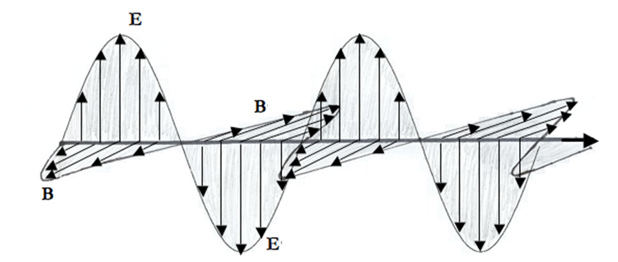
Thus, we arrive at the solution of the Maxwell's equations that corresponds to an electromagnetic wave traveling towards the positive \(x\)-axis. There are two waves, one for \(E_y\) and the other for \(B_z\) that travel at speed \(v=1/\sqrt{\mu_0\epsilon_0}\) and are described by the following functions.

\begin{align} \amp E_y(x,t) = E_0\cos\left[ k(x - vt) \right]\label{eq-plane-wave-Ey}\tag{45.4.14}\\ \amp B_z(x,t) = \frac{E_0}{v}\cos\left[ k(x - vt) \right]\label{eq-plane-wave-Bz}\tag{45.4.15} \end{align}

Subsection 45.4.3 Wavelength and Wavenumber

This solution is also called the plane wave solution. The meaning of the constant \(k\) can be gleaned by thinking of \(E_y\) as a function of \(x\) for a fixed \(t\text{,}\) say \(t=0\text{.}\) The distance \(\Delta x = \lambda\) over which the wave repeats itself is called the wavelength of the wave.

\begin{equation*} E_y(x,0) =E_y(x+\lambda,0)\ \ \Longrightarrow\ \ E_0\cos\left[ k\; x \right] = E_0\cos\left[ k\; (x+\lambda) \right]. \end{equation*}

This equation can be stratified if \(k\) and \(\lambda\) are related in a particular way.

\begin{equation*} k\lambda = 2n\pi,\ \ n = 0, \pm 1, \pm 2, \cdots \end{equation*}

Since \(\lambda \ne 0\text{,}\) the smallest \(|n|\) is 1 and we write the relation between the wavenumber and the wavelength as

\begin{equation*} k = \frac{2\pi}{\lambda}. \end{equation*}

The SI unit of wavelength is meter and that of the wave number radians per meter. The constant \(k\) is called the wavenumber and corresponds to the number of wavelengths (meters) of a wave that can fit in a distance of \(2\pi\) meters.

Subsection 45.4.4 Time Period and Frequency

In a plane wave, electric field at any one space point oscillates sinusoidally between \(+E_0\) and \(-E_0\text{.}\) For instance, if you place a detector at the origin, the \(y\)-component of the electric field on the detector will oscillate between the values \(+E_0\) and \(-E_0\text{.}\) The time period \(T\) of oscillations is obtained by looking at the repeat time for these oscillations.

\begin{equation*} E_y(0,t) =E_y(0,t+T)\ \ \Longrightarrow\ \ E_0\cos\left[ k\;v\;t \right] = E_0\cos\left[ k\;v\;(t+T)) \right]. \end{equation*}

Therefore,

\begin{equation*} kvT = 2n\pi,\ \ n = 0, \pm 1, \pm 2, \cdots \end{equation*}

Since \(T \ne 0\text{,}\) the smallest repeat time is the time period.

\begin{equation*} T= \frac{2\pi}{kv} = \frac{\lambda}{v}. \end{equation*}

The frequency \(f\) of oscillations is the number of oscillations that occur in a unit time. Therefore, the frequency \(f\) is equal to the inverse of time period \(T\text{.}\) This gives us the fundamental wave relation for the electromagnetic wave also.

\begin{equation*} \lambda f = v. \end{equation*}

Often an angular frequency \(\omega\) defined as follows is more useful in calculations.

\begin{equation*} \omega = 2\pi f. \end{equation*}

The wave functions are commonly written using \(k\) and \(\omega\) rather than \(k\) and \(v\) or some other constants. For instance, the \(E_y\) electric field traveling towards the positive \(x\)-axis given above will be written as

\begin{equation*} E_y(x,t) = E_0 \cos(kx-\omega t). \end{equation*}

Another common practice is to write the wave function to show the wavelength and frequency in the formula itself.

\begin{equation*} E_y(x,t) = E_0 \cos\left(2\pi\frac{x}{\lambda}-2 \pi f t\right). \end{equation*}

Subsection 45.4.5 Transverse Nature of Electromagnetic Waves in Vacuum

In the above subsection, we looked at a particular direction of wave. We found that when the wave was traveling towards the positive \(x\)-axis with the electric field pointed towards the positive \(y\)-axis and the magnetic field vector pointed towards the positive \(z\)-axis. This wave has the directions of the electric and magnetic fields in a plane perpendicular to the direction of the propagation of the wave as shown in Figure 45.4.2. This type of wave is called a transverse wave since the oscillations of the wave occur in the plane normal to the propagation. This is a general property of the electromagnetic waves in vacuum and in most materials, but not in all materials.

Figure 45.4.2. A plane transverse electromagnetic wave traveling in the \(+x\) direction. Solid lines are electric field \(\vec E\) and dashed lines the magnetic field \(\vec B\text{.}\) The direction of the vector fields at any point are perpendicular to each other and to the direction of the wave propagation.

To illustrate the general nature of the electromagnetic wave in vacuum, let us examine the relation between electric and magnetic waves traveling in an arbitrary direction. Let the arbitrary direction be denoted by a unit vector \(\hat u\) in a three-dimensional space. Consider an electric field vector wave traveling in vacuum given by the following function.

\begin{equation*} \vec E(\vec r, t) = \vec E_0 \cos(k\hat u\cdot \vec r - k c t+\phi), \end{equation*}

where \(\vec E_0\) is a constant vector with fixed magnitude and direction, \(k\) the wavenumber and \(c\) the speed. We are writing \(kc\) for \(\omega\) here to simplify the calculation below. The associated magnetic field vector wave will be

\begin{equation*} \vec B(\vec r, t) = \vec B_0 \cos(k\hat u\cdot \vec r - k c t+\phi), \end{equation*}

Now, we use the Maxwell's equations to find the relation between the directions of the three vectors, \(\vec E_0\text{,}\) \(\vec B_0\) and \(\hat u\text{.}\) Making the necessary calculations on the Faraday's law in the differential form leads to

\begin{equation*} -\hat u \times \vec E_0 = c \vec B_0. \end{equation*}

This says that \(\vec B_0\) is perpendicular to the plane of \(\vec E_0\) and \(\hat u\text{.}\) A similar calculation using the Ampere-Maxwell's law gives

\begin{equation*} \hat u \times \vec B_0 = -\frac{1}{c}\vec E_0. \end{equation*}

This says that \(\vec E_0\) is perpendicular to the plane of \(\vec B_0\) and \(\hat u\text{.}\) The two results leads to an unmistakeable conclusion that the three vectors \(\vec E_0\text{,}\) \(\vec B_0\) and \(\hat u\) are mutually perpendicular to each other.

\begin{equation*} \vec E_0 \perp \vec B_0;\ \ \hat u \perp\vec E_0;\ \ \hat u\perp\vec B_0. \end{equation*}

You can show that the direction of propagation \(\hat u\) is in the direction of the vector obtained from the cross product \(\vec E_0\times\vec B_0\text{.}\)

\begin{equation*} \text{Direction of propagation = The direction of }\ \vec E_0\times\vec B_0. \end{equation*}

Subsection 45.4.6 The Electromagnetic Spectrum

A wide range of electromagnetic waves have been either found in nature or produced in the laboratory. The collection of all EM waves is called the electromagnetic spectrum. They are usually categorized in various sub-ranges or bands as shown in Figure 45.4.3. Note the all important visible light occupies a minuscule band compared to the available EM spectrum.

Figure 45.4.3. The electromagnetic spectrum. The names of the bands and corresponding frequencies are given below the double line. Above the band some representative wavelengths in vacuum are given. Note that the boundaries between different bands are arbitrary.

The frequency of an electromagnetic wave is same as the frequency of vibrating charges that produce it. Hertz's waves had a frequency of about \(10^6\) cycles per second. These waves are now called radio waves. The visible light is also an electromagnetic wave but with considerably higher frequency than the radio waves. Visible light have frequency approximately between \(4 \times 10^{14}\) Hz (red) and \(7.5 \times 10^{14}\) Hz (violet) compared to the radio waves that have frequency less than \(10^8\) Hz.

The electromagnetic waves of frequency as high as \(10^{10}\) Hz are usually produced in the laboratory using a similar setup used by Hertz. It consists of an antenna upon which an oscillating voltage is applied which radiates electromagnetic waves. The EM waves of higher frequencies are not produced in the laboratory by this method. You can see from the fundamental wave relation that a higher frequency would correspond to a lower wavelength. To produce a visible light of frequency \(4 \times 10^{14}\) Hz, you would need an antenna less than one micrometer in length and a circuitry that can oscillate at \(4 \times 10^{14}\) Hz, both of which are not currently available.

The electromagnetic waves of higher frequencies are instead generated in natural processes of emission from atoms, molecules and nuclei. When an atom makes a transition from a higher energy state of energy \(E_1\) to a lower energy state of energy \(E_2\text{,}\) it emits a particle of light, called photon, corresponding to the frequency \(f\) of light given by the following energy balance equation:

\begin{equation*} h f = E_1-E_2, \end{equation*}

where \(h\) is the Planck constant. A schematic picture of the production of light in an atomic energy level transition is shown in Figure 45.4.4.

Figure 45.4.4. The atomic transition from a higher state to a lower state is accompanied by the emission of a particle of light called photon.

Subsection 45.4.7 Energy and Intensity of EM Waves

Traveling waves transport energy without actually moving particles. Therefore, you can think of an electromagnetic wave in terms of the flow of the electromagnetic energy. Consider the electromagnetic plane wave solution for electric and magnetic field waves in vacuum we found above. For a wave traveling in the direction of the positive \(x\)-axis with the phase constant \(\phi=0\) we had the following for the \(E_y\) and \(B_z\) waves.

\begin{align*} \amp E_y(x,t) = E_0\cos\left[ k(x - ct) \right]\\ \amp B_z(x,t) = \frac{E_0}{c}\cos\left[ k(x - ct) \right] \end{align*}

The other components of the electric and magnetic fields are zero in this solution. The energy per unit volume, or energy density (\(u\)), contained in these waves can be calculated by summing the energy in the electric and magnetic fields.

\begin{align} u(x,t) \amp = u_E + u_B = \frac{1}{2}\epsilon_0\vec E\cdot\vec E + \frac{1}{2\mu_0}\vec B\cdot\vec B.\notag\\ \amp = \epsilon_0 E_0^2\cos^2\left[ k(x - ct) \right] \label{eq-em-energy-den-1}\tag{45.4.16} \end{align}

Thus, the energy density moves along with the electric and magnetic waves in a similar manner as the waves themselves except that the wavelength is now half as much and the frequency twice as much because of the square of the cosine, which can be converted to a cosine by the double-angle trig formula. One might say that you also have a wave of electromagnetic energy density.

We can figure out the rate of the transport of energy by considering what happens in a small time interval \(\Delta t\text{.}\) As shown in Figure 45.4.5 the energy contained in a box of length \(c\Delta t\) and cross-sectional area \(A\) will pass through the cross-sectional plane in the interval \(\Delta t\text{.}\)

Figure 45.4.5. The energy \(uAc\Delta t\) contained in the electric and magnetic fields of the electromagnetic wave in the the volume \(Ac\Delta t\) will pass through the area \(A\) in time \(\Delta t\text{.}\)
\begin{equation*} \text{The energy passing through area }A \text{ in time }\Delta t = u\times \text{volume} = u A c \Delta t. \end{equation*}

The energy per unit area per unit time passing through plane perpendicular to the wave, called the power flux and denoted by \(S\text{,}\) can be calculated by dividing the energy by the area \(A\) and the time interval \(\Delta t\text{.}\)

\begin{equation*} \text{Power flux,}\ S = \frac{\text{Energy passing area }A \text{ in time }\Delta t}{A\Delta t} = u\; c. \end{equation*}

The flux of power at any place also fluctuates in time as can be seen by substituting u from Eq. (45.4.16).

\begin{equation*} S(x,t) = c\epsilon_0 E_0^2\cos^2\left[ k(x - ct) \right] \end{equation*}

Since the frequency of visible light is very high, of the order of \(10^{14}\) Hz, the power flux for visible light through any area will be an extremely rapidly varying quantity. Most measuring devices as well as our eyes cannot respond so quickly and in most situations only an average over many cycles is observed. The quantity obtained by time-averaging the power flux is called the intensity or irradiance \(I\) of the electromagnetic wave.

\begin{equation*} \text{Intensity,}\ I = \left\langle S \right\rangle_{\text{time-average}}. \end{equation*}

The time-averaging of power flux is easily obtained by noting the following mathematical result. (Here \(T\) is one period.)

\begin{equation*} \frac{1}{T}\int_{0}^{T}\ \cos^2\left(2\pi\frac{t}{T} \right) dt. \end{equation*}

Hence, the intensity of light moving at speed c in vacuum is found to be

\begin{equation*} I = \langle S(x,t)\rangle =\frac{1}{2} c\epsilon_0 E_0^2, \end{equation*}

where the angle brackets \(\langle\cdots\rangle\) stands for the time averaging operation.

Remark 45.4.6. Poynting Vector.

Note that the amount of energy crossing a given area also depends upon the orientation of the area relative to the direction of light. To take the direction into account a power flux vector \(\vec S\text{,}\) also called the Poynting vector, is introduced by the following defining equation.

\begin{equation*} \vec S = \frac{1}{\mu_0}\vec E\times \vec B. \end{equation*}

The cross-product of \(\vec E\) and \(\vec B\) points in the direction of the propagation of the electromagnetic wave. Therefore, the Poynting vector \(\vec S\) points in the direction of the propagation of the electromagnetic wave.

We can write the power flux through any arbitrarily oriented area and arbitrary electromagnetic wave in terms of the Poynting vector. Consider dividing the surface into small patches of area vector \(\Delta\vec A\text{.}\) Now, we calculate the power through each patch, and then sum up the contributions. Let \(\vec S\) be the average Poynting vector over a patch of area vector \(\Delta\vec A\text{,}\) then the power crossing this area elements will be given by the projection of \(\vec S\) on \(\Delta\vec A\) times the area, which can be written in terms of the scalar product of the two vectors.

\begin{equation*} \text{Power through the area element} = \vec S\cdot \Delta\vec A. \end{equation*}

The total power crossing any surface is equal to the sum of the contributions from all patches. The sum over infinitesimal patches leads to the following integral formula, which is the integral for the flux of vector fields.

\begin{equation*} \text{Power through any surface} = \int_{\text{surface}}\vec S\cdot d\vec A. \end{equation*}

Subsection 45.4.8 Momentum of EM Wave and Radiation Pressure

Imagine an electromagnetic wave incident on a metal. The electrons of the surface atoms will be accelerated by the electric field in the wave. In the case of the electromagnetic wave with electric field pointed towards positive \(y\) axis, electrons will accelerate in the negative \(y\) direction. At that instant, magnetic field of EM wave would be in the positive \(z\)-axis. This will result in a magnetic force on the electrons in the direction of the positive \(x\)-axis, which is the direction of the electromagnetic wave. Thus, the metal will experience a net force in the direction of the electromagnetic wave.

Maxwell calculated force per unit area, called the radiation pressure, \(P_{\text{rad}}\text{,}\) applied by an electromagnetic wave on a perfectly absorbing surface and found it to be equal to the energy density of the wave.

\begin{equation} P_{\text{rad}} = u.\ \ \text{(Perfect abosorber)}\label{eq-rad-pres-1}\tag{45.4.17} \end{equation}

If the material is perfectly reflecting such as the metal surface and if the incidence is along the normal to the surface, then the pressure exerted will be twice as much since the momentum direction will reverse upon reflection and conservation of momentum will imply

\begin{equation} P_{\text{rad}} = 2u. \ \ \text{(Perfect reflector)}\label{eq-rad-pres-2}\tag{45.4.18} \end{equation}

Do not confuse \(P_{\text{rad}}\) with the power. Let's see if the units are right.

\begin{equation*} [u] = \frac{\text{J}}{\text{m}^3} = \frac{\text{N.m}}{\text{m}^3} = \frac{\text{N}}{\text{m}^2} = \text{unit of pressure!} \end{equation*}

Equations (45.4.17) and (45.4.18) give instantaneous pressure, but since energy density of EM wave oscillates rapidly, we are usually interested in the time-averaged quantity, as was the case with our interest in intensity. The time average of radiation pressure can be expressed in terms of intensity also.

\begin{equation*} P_{\text{ave}}^{\text{rad}} = \begin{cases} I/c \amp \quad \text{Perfect absorber}\\ 2I/c \amp \quad \text{Perfect reflector} \end{cases} \end{equation*}

The electric field of an electromagnetic wave traveling in vacuum is described by the following wave function.

\begin{equation*} \vec E = \hat j\ (5\ \textrm{N/C})\cos\left(k\: x - 6\times 10^{9}\: t + 0.4 \right) \end{equation*}

where \(k\) is the wavenumber in rad/m, \(x\) in m, \(t\) in sec. Find the following quantities.

  1. Amplitude.
  2. Frequency.
  3. Wavelength.
  4. Phase constant.
  5. The direction of the travel.
  6. The associated magnetic field wave.
  7. The Poynting vector of the electromagnetic wave.
  8. The intensity of the electromagnetic wave.
Hint

Use definitions.

Answer

(a) \(5\ \textrm{N/C} \text{,}\) (b) \(3.77\times 10^{10}\:\textrm{Hz}\text{,}\) (c) \(7.96\:\textrm{mm}\text{,}\) (d) \(0.4\text{ rad}\text{,}\) (e) positive \(x\)-axis, (f) \(\vec B = \hat k\ \left(\dfrac{5\ \textrm{N/C}}{3\times 10^{8}\:\textrm{m/s}}\right)\cos\left(0.8\text{ mm}^{-1}\: x - 6\times 10^{9}\text{ s}^{-1}\, t + 0.4 \right)\text{,}\) (g) \(\hat i\ \:\dfrac{1}{\mu_0}\: c\: E_0^2\:\cos^2\left(k\: x - 6\times 10^{9}\: t + 0.4 \right) \text{,}\) where \(E_0 = 5\ \textrm{N/C}\) and \(c=3\times 10^8\:\textrm{m/s}\text{,}\) (h) \(33.2\:\textrm{mW/m}^2\text{.}\)

Solution

We will read off the answer from the given expression for the wave function, \(\vec E = \hat j\ (5\ \textrm{N/C})\cos\left(k\: x - 6\times 10^{9}\: t + 0.4 \right)\)

  1. Amplitude, \(E_0 = 5\ \textrm{N/C}\text{.}\)

  2. Frequency, \(f\) = \(2\pi\times 6\times 10^{9} = 3.77\times 10^{10}\:\textrm{Hz}\text{.}\)

  3. Wavelength = \(\dfrac{c}{f} = 7.96\:\textrm{mm}\text{.}\)

  4. Phase constant = \(0.4\text{ rad}\text{.}\)

  5. The direction of the travel is towards the positive \(x\)-axis.

  6. The associated magnetic field wave. The argument of the oscillating part will be same for the \(\vec E\) and \(\vec B\) fields. The magnitude of the \(\vec B\) field will be \(1/c\) of the magnitude of the \(\vec E\) field and the direction of the \(\vec B\) will be perpendicular to the direction of the \(\vec E\) field. Using the right-hand rule, we deduce that, for a wave moving towards the positive \(x\)-axis, when \(E\)-field is pointed towards the \(y\)-axis, the electric fiend will be pointed towards the \(z\)-axis. Therefore, we will have the following for the magnetic field wave.

    \begin{equation*} \vec B = \hat k\ \left(\dfrac{5\ \textrm{N/C}}{3\times 10^{8}\:\textrm{m/s}}\right)\cos\left(k\: x - 6\times 10^{9}\: t + 0.4 \right), \end{equation*}

    where \(k = 2\pi/\lambda = 0.8\text{ mm}^{-1}\) with \(\lambda = 7.96\text{ mm}\) as found above.

  7. The Poynting vector of the electromagnetic wave will be given by

    \begin{equation*} \vec S = \dfrac{1}{\mu_0}\: \vec E\times \vec B = \hat i\ \:\dfrac{1}{\mu_0}\: c\: E_0^2\:\cos^2\left(k\: x - 6\times 10^{9}\: t + 0.4 \right), \end{equation*}

    where \(E_0 = 5\ \textrm{N/C}\) and \(c=3\times 10^8\:\textrm{m/s}\text{.}\)

  8. The intensity of the electromagnetic wave is the time-average of the power flux \(S\) given by the magnitude of \(\vec S\text{.}\) We find

    \begin{equation*} I = \dfrac{1}{2}\:c\:\epsilon_0\:E_0^2 = 33.2\:\textrm{mW/m}^2. \end{equation*}

A radio wave (which is an EM wave) has a frequency of \(12 MHz\text{.}\) What is its wavelength in vacuum?

Hint

Definition.

Answer

\(25 m\text{.}\)

Solution

Since speed of the wave is \(c = 3\times 10^{8}\:\textrm{m/s}\text{,}\) we will get

\begin{equation*} \lambda = \dfrac{c}{f} = \dfrac{3\times 10^{8}\:\textrm{m/s}}{12\times 10^{6}\:\textrm{Hz}} = 25\:\textrm{m}. \end{equation*}

A laser light of power \(3\text{ W}\) is spread evenly across the cross-section of the beam of diameter \(2\text{ mm}\text{.}\) When the laser light is incident on a perfectly reflecting surface of a spherical particle of diameter \(1.5 \text{ mm}\) in vacuum, the particle is observed to be suspended in space. Find the density of the particle.

Hint

The force due to the radiation pressure is able to balance the force of gravity.

Answer

\(0.2\; \text{kg/m}^3\text{.}\)

Solution

Here, the force due to the radiation pressure is able to balance the force of gravity. Let \(\rho\) be the desired density of the spherical particle, \(R\) its radius, \(A\) the area of cross-section, and \(V\) its volume. Let \(P\) be the radiation pressure at the site of the particle. The balancing of forces yields the following relation.

\begin{equation*} P A = \rho V g. \end{equation*}

Here the radiation pressure acts on the cross-section area of the particle, which is simply a circle of radius \(R\text{,}\) and the volume of the particle is just the volume of a sphere.

\begin{equation*} P \pi R^2 = \rho \frac{4}{3}\pi R^3 g. \end{equation*}

Hence the required density is

\begin{equation*} \rho = \frac{3}{4}\; \frac{P}{gR}. \end{equation*}

Now, we put the numerical values given here.

\begin{align*} \amp R = 0.75\; \text{mm} = 7.5\times 10^{-4}\; \text{m} \nonumber\\ \amp g = 9.81\; \text{m/s} \\ \amp P =2\frac{I}{c} = 2\times \frac{3\; \text{W}}{\pi\left( 1.0\times 10^{-3}\; \text{m}\right)^2 }\times \frac{1}{3\times 10^8\; \text{m/s}} = 2\times 10^{-3}\; \text{Pa}. \end{align*}

Hence, the density of the material of the particle is

\begin{equation*} \rho = 0.2\; \text{kg/m}^3. \end{equation*}

It is interesting to compare the density found to the density of aluminum, a light metal, which has the density \(2700 \text{ kg/m}^3\text{.}\) Clearly, one will need a very powerful laser to suspend an ordinary material.