Physics Bootcamp

Subsection 59.2.1 Apparent Magnitude and Flux

Although, the flux \(F_m\) would provide a reasonable scale to classify apparent brightness of stars, the system used by Astronomers is based on a logarithmic scale because our visual perception is actually a logarithmic detector. The designation brightness of stars dates back to Hipparchus of Nicaea who cataloged 1000 stars in about 130 B.C. and introduced a system of six magnitudes for classifying them. Hipparchus assigned magnitude 1 to the brightest stars, 2 to the next group, and so on, finally 6 to the stars that were barely visible to the naked eye without the aid of a telescope.

The system of Hipparchus was systematized and made more quantitative by Norman Pogson in 1856, who gave the brightness of the brightest star a factor of 100 compared to the brightness of the faintest star and then divided the factor 100 into equal factors for each magnitude. This gave him a factor of 2.512 for each magnitude.

Thus, a star of magnitude 1 was 2.512 times as bright as a star of magnitude 2, which in turn was 2.512 times as bright as a start of magnitude 3, and so on. Thus, we have five factors of 2.512 between magnitudes 1 and 6.

The bright stable star Vega is taken to be the reference zero-point of the magnitude scale. This gives the following formula for apparent magnitude \(m\) of a star with respect to the apparent magnitude \(m_0 = 0\) for Vega.

Of course, you can write this equation in terms of the luminosities of the two stars by multiplying the two fluxes by a common factor of \(4\pi r\text{.}\)

Using this equation you can compare the magnitudes \(m_1\) and \(m_2\) of any two stars. Subtracting the formulas of \(m = m_1\) and \(m=m_2\) cancels out any reference to the reference star and we find

Thus, if we have a star of magnitude 1 and another of magnitude 6, then by definition, the ratio of their fluxes should be 100.

We can also use Eq. (59.2.5) to write the absolute magnitude \(M\) and apparent magnitude \(m\) of a star with \(M\) being the magnitude at a distance of 10 pc from the star. To convert the ratio of the fluxes we use Eq. (59.2.3). Thus,

The quantitative method provides us with a more precise way to classify the apparent brightness. With improvement in observation technology, we can make measurements on extremely dim stars and use the magnitude scale to refer to them. For instance, Hubble telescope could observe stars with magnitude 30, which \(2.5^{24} = 4 \times 10^9\) times fainter than the faintest star visible to the naked eye. On this scale, the moon has \(m = -12.74\) and the sun \(m = -26.71\text{.}\) The brightest star in the sky, Sirius has \(m = -1.4\text{.}\)

Subsection 59.2.2 Temperature of Stars

In the early 1900s, stars were grouped into a series of spectral types based on the types and strengths of the spectral absorption lines. The spectral types are labeled by the letters, O, B, A, F, G, K, M. Often a mnemonic is used to remember this sequence: Oh Be A Fine Girl/Guy, Kiss Me! Our Sun is a G type star. Much finer classification is also used, but we will not discuss them here. The absorption lines are primarily determined by the surface temperature of the star, with O type star having the highest temperature, B the next hot, and so on.

The spectra of stars contain evidence of the chemical content of the stars as well as the temperature at the surface of the stars. The light coming from stars has absorption and emission lines corresponding to elements in the star. Elements are excited at different temperatures and lines from different elements become strongest at different temperatures. Thus, the absoption and emissions lines of a star are indicative of the temperature of the star. Table 59.2.4 and Table 59.2.5 lists some characteristics of different types of stars.

We can assign a surface temperature to a star if we assume that the emission of the star closely resembles that of a blackbody spectrum. The nuclear processes at the outer layer of a star tends to thermalize the photons before they are emitted and are close to the blackbody spectum. Thus, the flux \(F_{*}\) at the star surface would be given by Stefan-Boltzmann law.

where \(T\) is the temperature of the blackbody, \(\sigma = 5.67 \times 10^{−8} \textrm{W m}^{−2}\textrm{K}^{−4}\text{,}\) the Stefan-Boltzmann constant, and \(F_{*}\) is related to the luminosity and radius \(r_*\) of the star as

From Eqs. (59.2.7) and (59.2.8)

The temperature of a star can also be obtained from the wavelength \(\lambda_{\textrm{max}}\) at which the spectrum of the star has the maximum intensity by applying Wien's displacement law.

From Eqs. (59.2.7) and (59.2.10), we find that a determination of the maximum of the spectrum can be used to determine the flux at the surface of the star.

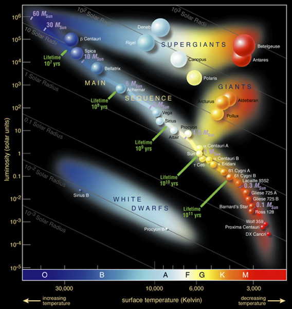
Subsection 59.2.3 The Hertzsprung-Russell Diagram

During 1905-1913, the Danish astronomer Ejnar Hertzsprung and the American astronomer Henry Norris Russell independently introduced a plot of stars according to their luminosity and spectral type, or equivalently, the surface temperature which has turned out to be extremely valuable tool for thinking about stars of various types. The diagram is called Hertzsprung-Russell or H-R diagram.

In the H-R diagram, shown in Figure 59.2.7 the vertical axis corresponds to increasing luminosity and the horizontal axis to the decreasing temperature following Russell's choice. The top left corner corresponds to high luminosity and high temperature and the bottom right corner to the lowest luminosity and lowest temperature. Each star is placed on the diagram according to its luminosity and temperature. As more and more stars are placed in the diagram, only certain areas of the diagram fill up while other areas remain empty with very few stars if any. Different parts of the diagram that fill up correspond to different types of stars.

The Sun is near the middle of the H-R diagram in a band of stars that goes roughly from the top left corner to the bottom right corner. These stars are called the main-sequence stars. The main-sequence stars get their energy from burning hydrogen into helium similar to the process in the Sun. The Red Giants and Super Giants are very massive stars. They occupy a region above the main-sequence in the H-R diagram. The burnt out stars, so-called white dwarfs, occupy the bottom left side of the diagram.