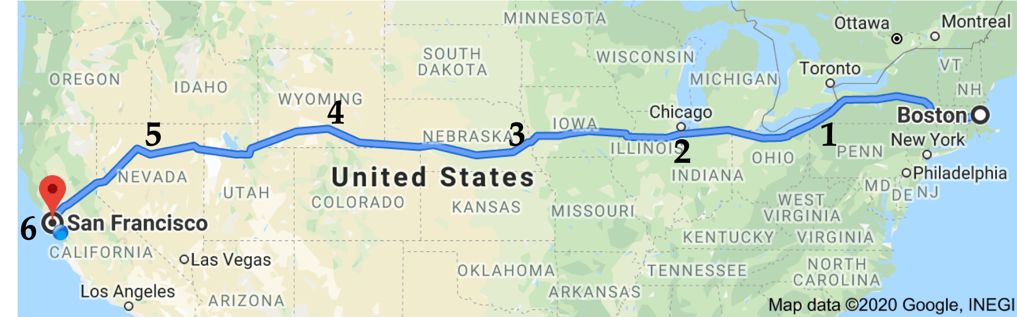
Tracing a motion on a diagram is the most basic way of representing motion. If you have taken a road trip or train journey, you are already familiar with this idea. You do this by marking time at various points along your path. This would be your motion diagram. For instance, Figure 2.3 shows motion diagram for a road trip from Boston (USA) to San Framcisco (USA), where points on the map are marked every 24 hours.
Figure2.3.A trip from Boston to San Francisco with each day marked is an example of a motion diagram. Credits: https://maps.google.com.
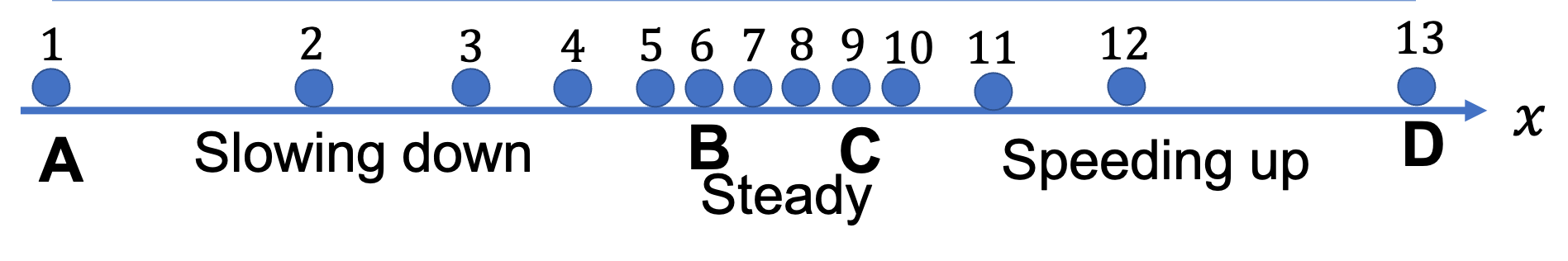
Often we mark position at regular time intervals so that we can easily understand the motion diagram immediately qualitatively, such as where an object is moving steadily, or where speeding up, or where slowing down. For instance, from motion diagram in Figure 2.4, it is immediately obvious that the car is slowing between A and B, moving at a steady pace between B and C, and speeding up betwen C and D.
Figure2.4.A motion diagram shows position at regular intervals of time - you might think of dots marked every second. The object is slowing between A and B, speeding up between C and D, and is steady between B and C.
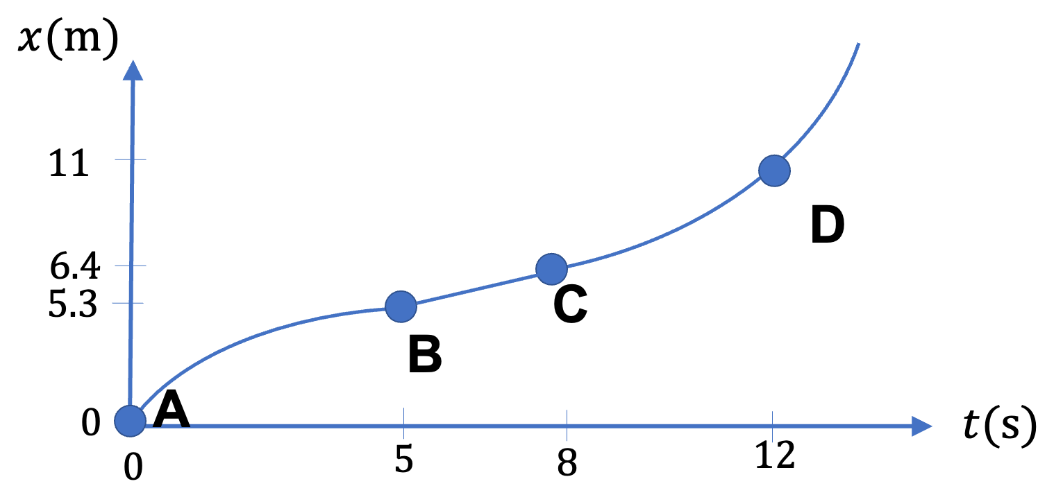
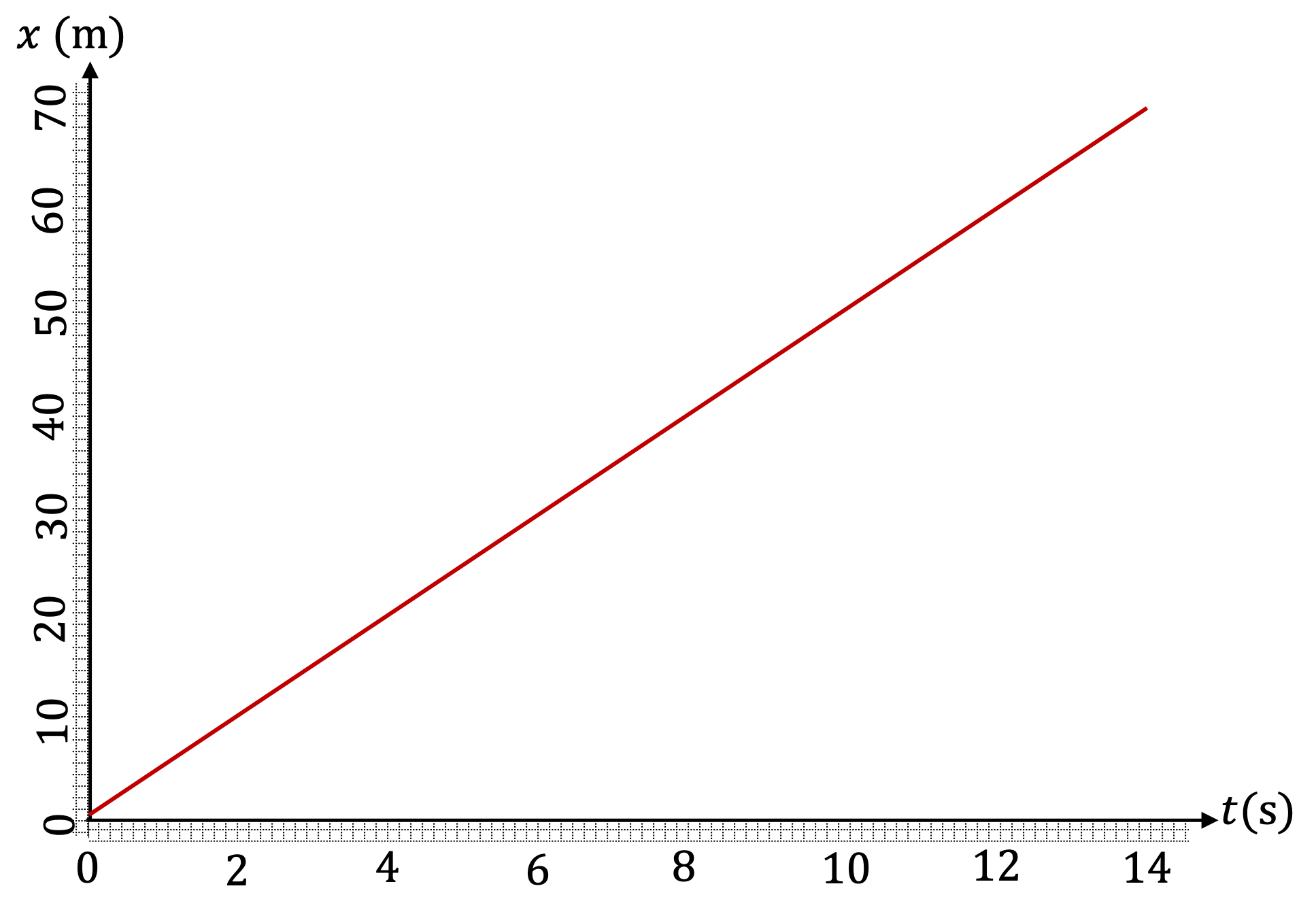
If you were moving on a straight path, as in Figure 2.4, you could view the motion occuring on a Cartesian axis, say the \(x \) axis. Your markings would then give \(x \) coordinates at various times \(t \text{.}\) We can fit (i.e., use interpolation between the data points by smooth curve) these data points to obtain a position as a function of time, namely, \(x(t) \text{,}\) as shown in Figure 2.5. The benefit of thinking in terms of function \(x(t)\) is that you can do further analysis of motion. You will see that this function gives us analytic definitions of velocity and acceleration, two important characterizations of motion.
Figure2.5.The \(x \) versus \(t \) plot corresponding to the motion in Figure 2.4.
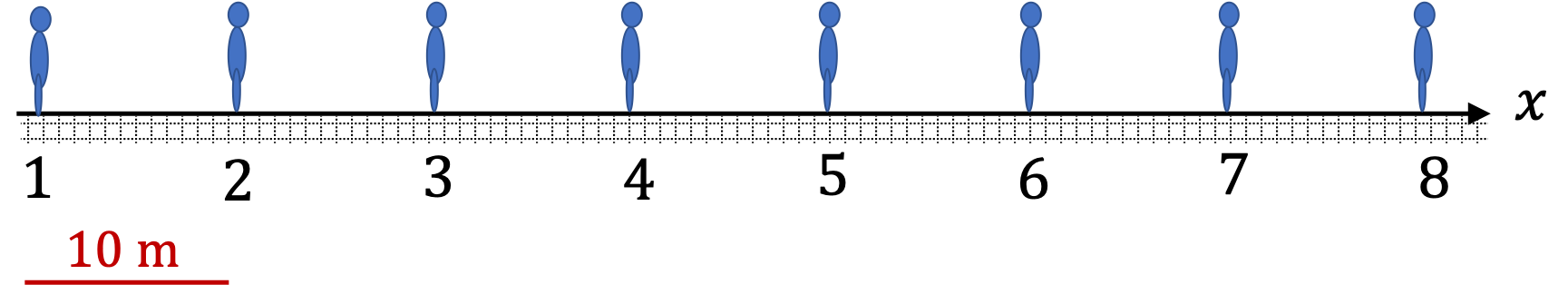
Example2.6.A Boy Running On a Straight Track Uniformly.
Figure 2.7 shows a boy running on a straight track. The position of the boy is marked every 2 seconds. The line below the sketch shows the scale of length in the drawing.
(a) Draw \(x \) versus \(t \) representation on the motion diagram.
(b) Is the motion steady, slowing down, or speeding up? How can you tell?
(a) See solution. (b) Steady since covering same distance in same amount of time.
Solution1.a
We use the scale to figure out distances from where the boy is at point marked 1. The plot in Figure 2.8 shows \(x \) values along the ordinate and \(t \) values along the abscissa.
Steady since covering same distance in same amount of time. Also, steady since the plot of \(x \) vs \(t \) is a straight line.
Example2.9.From \(x \) Versus \(t \) Plot to Motion Diagram.
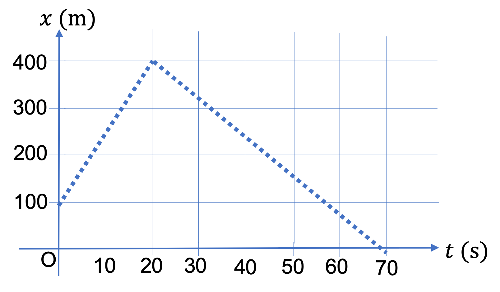
Figure 2.10 shows a plot of \(x \) versus \(t \text{.}\) Draw a motion diagram that will result in this plot. Show space scales and indicate value of time on your diagram.
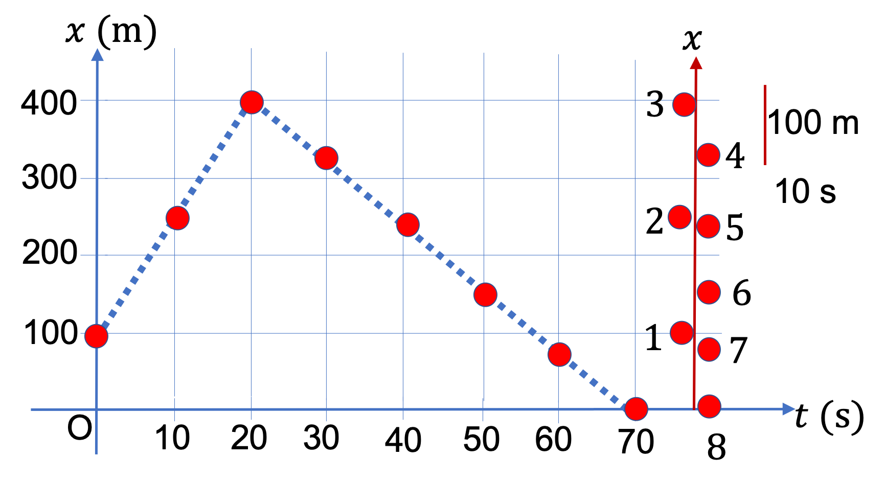
First we mark points on the ordinate axis at equal-time intervals. We choose to mark points separated by \(10\text{ s}\) intervals. These points are shown as dots in \(x\) vs \(t\) plot in Figure 2.11. Then we draw points on the \(x \) axis only to get the motion diagram, where we now label each point as 1, 2, 3, ..., which stand for the instants, with label 2 for 10 sec, label 3 for 20 sec, and so forth.
Figure2.11.Constructing a motion diagram (the line on the right side) from \(x\) vs \(t\) plot (the plot on the left side).
ExercisesExercises
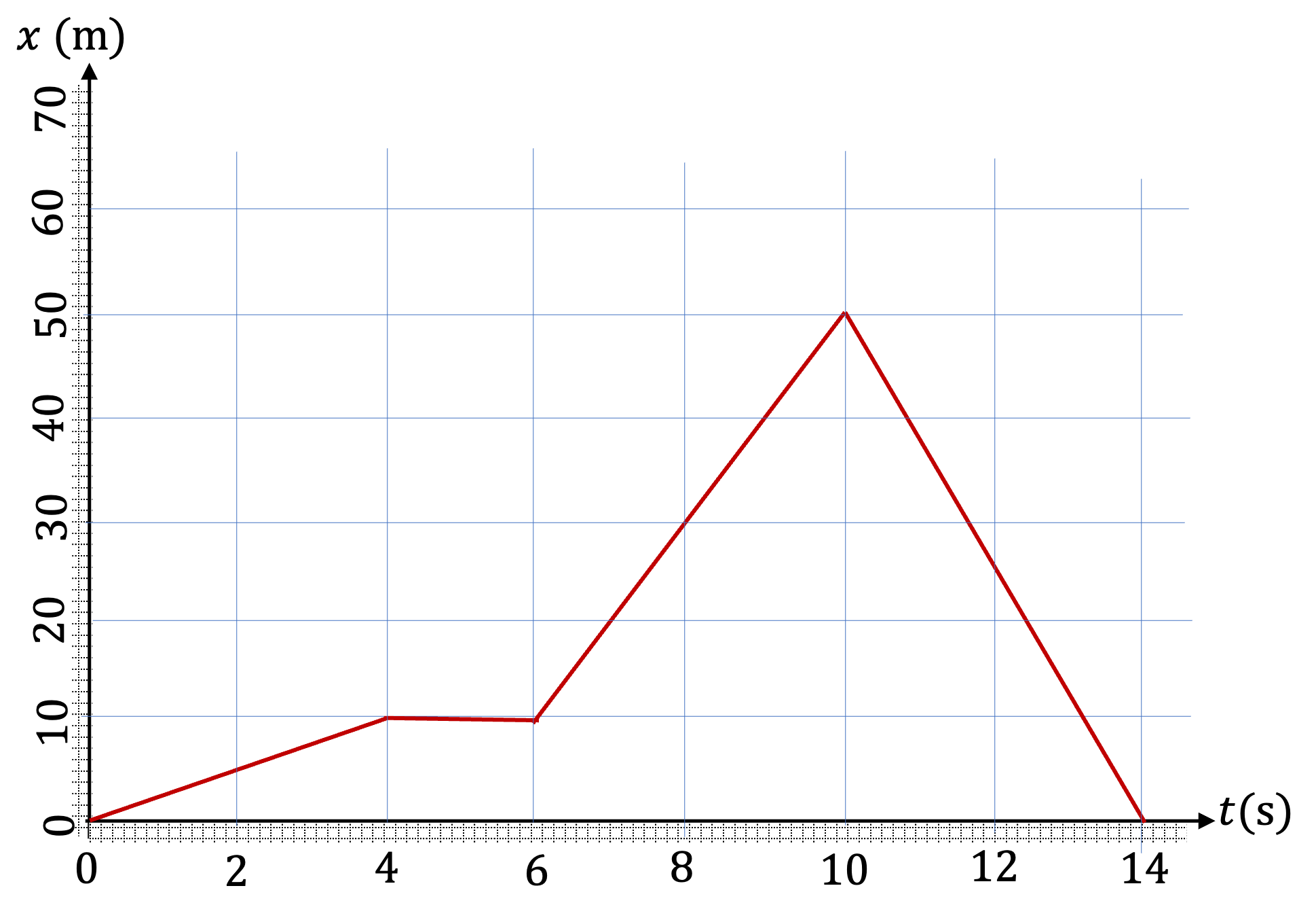
1.Practice with a Friend.
Figure 2.12 shows a plot of \(x \) versus \(t \text{.}\) Draw a motion diagram that will result in this plot. Show space scales and indicate value of time on your diagram.