Section 1.4 Uncertainty, Precision, Accuracy

Often when you measure the same quantity repeatedly you get different values. If spread of values is small, then we say that precision is high and when the spread is large, the precision is said to be low. Uncertainty in a measured quantity is quantitative statement of precision.

Usually, value of uncertainty is obtained by statistical analysis of the spread of the measured values. We will not be discussing these methods, but instead, take it as given by the experimenter. Thus, measurements of a quantity gives rise to two values: main value and uncertain amount. For instance, repeated length measurements of the same rod will give us main value \(L\) and uncertain amount \(\Delta L\text{.}\)

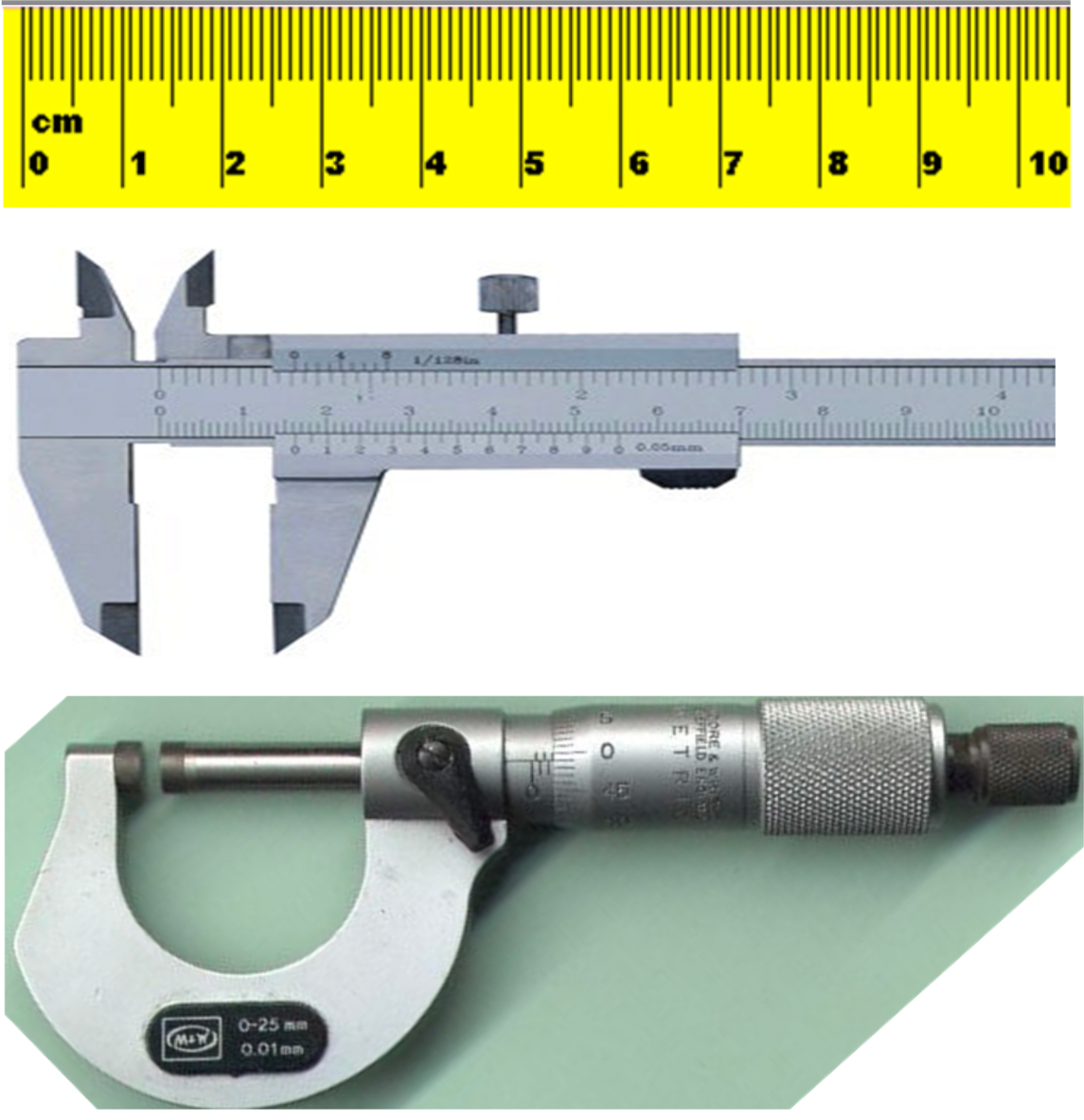
There is another meaning of precision - a value known to larger number of digits is also said to be more precise. For instance, if you measure thickness of a wire by using a millimeter-ruled ruler, you might get value up to about \(0.5\text{ mm}\text{,}\) but with a vernier caliper you could get precision up to \(0.01\text{ mm}\) and with a micrometer, may be even \(0.005\text{ mm}\text{.}\)

Figure 1.4.1.

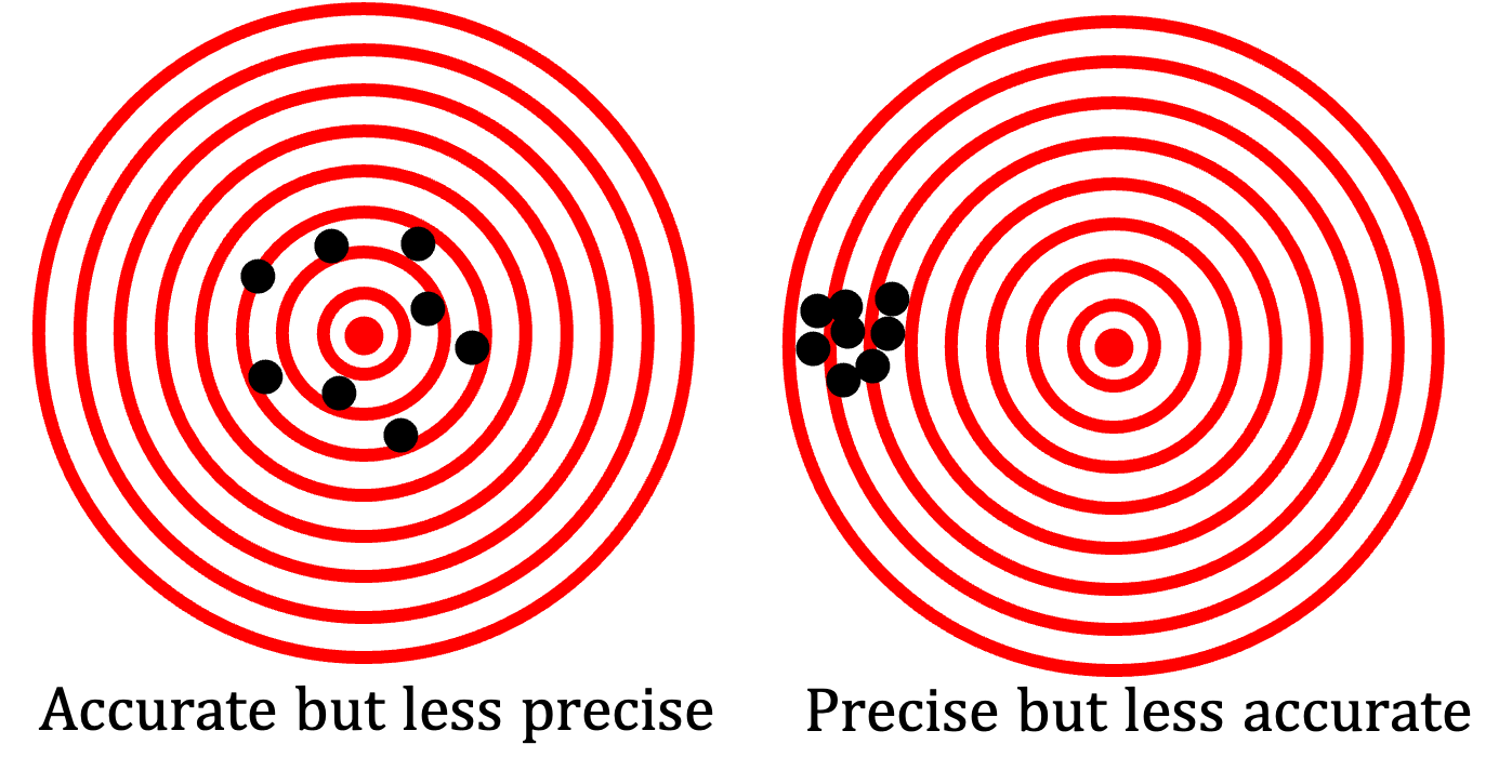
Accuracy is different. Accuracy refers to how close measured values are to some known value. You may have highly repeatable values but which are way off the known value. That will be the case of high precision and low accuracy.

Figure 1.4.2.

For instance, suppose you used a faulty watch and measured a period of a pendulum to be \(4.5\text{ s}\) but the actual value was \(4\text{ s}\text{.}\) That's \(12.5\%\) error and not very accurate.

A normal practice is to round off the uncertain amount to one non-zero digit and use that absolute uncertainty figure as a guide to round off the main number to the same precision level. So, if you somehow ended up with main amount \(2.57\text{ cm}\) with uncertain amount \(0.1\text{ cm}\text{,}\) you would use the precision of the uncertain amount and round off the main value to the same precision. Thus, this will become \(2.6\text{ cm}\) with uncertain amount \(0.1\text{ cm}\)

Why do we get spread in values of measured quantities? One or more factors may be at play.

  1. No measuring device is not capable to infinite precision.
  2. Object may have irregularities, e.g., if you are measuring length of a table, the edges of the table may not be sharp enough or length may vary along the table.
  3. You might not be able to reproduce the conditions exactly when you repeat measurement.
  4. You might make mistake by not making sure there are no obvious sources of error or carrying out a faulty procedure.

Subsection 1.4.1 Absolute and Relative Uncertainty

We report uncertainty in a measurement in one of two equivalent ways, called absolute uncertainty and relative uncertainty. To illustrate the difference, suppose, you measure thickness \(D\) of a wire by a Vernier caliper and want to report your answer as \(D=0.50\text{ mm}\) with an uncertainty of \(\Delta D = 0.01\text{ mm}\text{.}\) Here \(0.01\text{ mm}\) will be the absolute uncertainty. We report this using a plus minus sign.

\begin{equation} D \pm \Delta D = 0.50 \text{ mm} \pm 0.01 \text{ mm} = \left( 0.50 \pm 0.01 \right)\text{ mm}.\label{eq-absolute-uncertainty}\tag{1.4.1} \end{equation}

The problem with absolute uncertainty is that we do not know how bad the uncertainty is relative to the main value. You may be interested in uncertainty as a percentage of the main value - this is called relative uncertainty. In that case, you will divide absolute uncertainty by the main value to get relative uncertainty. In this example

\begin{equation*} \frac{\Delta D}{D} = \frac{0.01\text{ mm}}{0.50\text{ mm}} = 0.02. \end{equation*}

Relative uncertainty of \(0.02\) is \(2\%\text{.}\) We often speak of relative uncertainty as percentage error. Relative uncertainty is reported as

\begin{equation} D \pm \frac{\Delta D}{D}\% = 0.50 \text{ mm} \pm 2.0\%. \label{eq-relative-uncertainty}\tag{1.4.2} \end{equation}

Notice that you can easily go from absolute (Eq. (1.4.1) ) to relative (Eq. (1.4.2) ) and vice-versa. Practice with, say, from \(10.0 \text{ sec} \pm 5.0\% \) to absolute uncertainty.

Remark 1.4.3. Uncertainty and Accuracy.

The accuracy of a measurement does not refer to the precision of the measurement, but instead, to the closeness of the measured value to the “true value”, also called the accepted value. The accuracy is often expressed in percent error.

\begin{equation*} \text{Percent Error} = \frac{|\text{Accepted Value - Experimental Value}|}{ |\text{Accepted Value}| }\times100\%. \end{equation*}

Thus, if you measured the width of a metal plate to be \(5.7\text{ cm}\) while it was manufactured to the “exact” specification of \(6.0\text{ cm}\text{.}\) Then, your percent error will be \(5\%\) as obtained from the following calculation.

\begin{equation*} \text{Percent Error} = \frac{|6.0-5.7|}{|6.0|}\times100\% = 5\%. \end{equation*}

The causes of percent error may be a defect in the ruler or a faulty procedure of measurement.

Remark 1.4.4.

Although there is an uncertainty in every measurement, for the sake of brevity I will not be indicating any uncertainty in values given in problems or tables in this book. When an uncertainty is not specified, the general practice is to regard the last digit to be uncertain by one or two units. For example, if the length of a rod is given to be \(55.7\text{ cm}\) then it is usually assumed that the length is between \(55.6\text{ cm}\) and \(55.8\text{ cm}\) using one unit of the last digit as uncertainty. I will try to follow this practice when truncating the digits in numerical problems.

Subsection 1.4.2 Uncertainty in Calculations

Subsubsection 1.4.2.1 Significant Figures

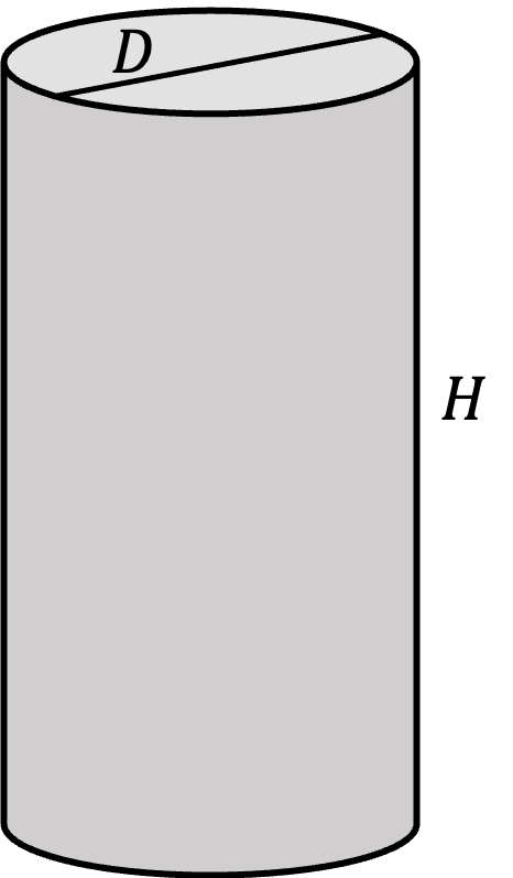
Suppose you measured diameter of a cylinder with main value \(D = 2.5\text{ cm}\) and uncertainty \(\Delta D = 0.1\text{ cm}\) and height \(H=5.23\text{ cm}\) with uncertainty \(\Delta H = 0.02\text{ cm}\text{.}\) What will be its volume? We would want main value \(V\) and uncertainty \(\Delta V\text{.}\) It is possible to propagate \(\Delta D\) and \(\Delta H\) to \(\Delta A\) by using Calculus. We will address that question in another section on propagation of uncertainty. Here, we want to address getting \(V\) to a reasonable number of digits, called number of significant figures, that respects the precision with which D and \(H\) were measured. We make use of a simple principle:

Figure 1.4.5.

Answer for a derived quantity cannot have more precision than the precision of the measured value. If we add or multiply or divide two quantities, the number of significant digits in the answer should equal lesser of the two quantities. By maintaining significant figures throughout a calculation we keep the precision of measured quantities in our derived quantities.

In our example since \(D\) was measured to two digits and \(H\) to three digits. Therefore, we expect \(V\) to have only two significant digits, i.e., we will round off \(V\) to two digits.

\begin{equation*} V = \frac{\pi}{4}D^2 H = \frac{\pi}{4}( 2.5\text{ cm})^2 \times 5.23 = 25.6727\Longrightarrow 26\text{ cm}^3. \end{equation*}

A more complete analysis will, of course, give you uncertainty \(\Delta V\) as well.

In numerical calculations where uncertainty is not explicitly stated it is assumed that the last digit displayed is uncertain. For instance, a measure quantity stated as \(786\) would imply that it has three significant figures. Integers with trailing zeros without a decimal at the end do not count in significant figures. Thus, \(78600\) still has three significant figures. But \(78600.\) has five significant figures.

Subsubsection 1.4.2.2 The Scientific Notation for Numbers

Writing physical numbers in the scientific notation helps with maintenance of significant figures in calculations. In scientific notation we use powers of 10 to write a decimal number with an additional requirment of writing the multiplier to have required number of significant figures. A number with \(n\) significant digits in scientific notation will have the following form.

\begin{equation*} d_1.d_2d_3\cdots d_n \times 10^{x}, \end{equation*}

with \(d_1\) a non-zero integer and all other \(d_i\) can be zero or non-zero digit. For instance, if a measured quantity was stated as \(786\text{,}\) we assume that it has three significant digits. We can then write this number in scientific notation as

\begin{equation*} 7.86 \times 10^{2}. \end{equation*}

Unlike non-scientific notation of numbers, trailing zeros on the right of decimal are considered significant. For instance, \(1.23\times 10^{5}\) is in scientific notation with three significant figures. Suppose you write this number as \(12.3\times 10^4\text{.}\) Although, it is the same number, but it is not in a scientific notation. Now, \(1.2300\times 10^{5}\) is numerically same as \(1.23\times 10^{5}\) but, as a scientific notation, they are not same since trailing zeros in \(1.2300\times 10^{5}\) as scientific notation are significant.

Following examples illustrate the standard scientific notation and the same numbers not in standard scientific notation.

\begin{align*} \amp \text{Scientific: } 1.5\times 10^{-3},\ \ 9.05\times 10^6,\ \ 9.050 \times 10^3.\\ \amp \text{Non-scientific: } 0.0015,\ \ 90.5\times 10^5,\ \ 9050. \end{align*}

Special Treatment of Zeros. Whether a zero in a number counts as a significant figure or not depends on the convenstion used to write that number. Thus, in \(0.00785\text{,}\) none of the zeros are significant since they are just placeholders. Its best to write this to three significant digits using the scientific notation: \(7.85\times 10^{-3}\text{.}\) How about trailing zeros on the right side, e/g., in \(7.8500\text{?}\) The two zeros on the right may or may not be significant; if we are additionally told is this number should be four significant figure, then it should be written as \(7.850\) and if it is supposed to be five significant figures, then \(7.8500\) is right. Finally, if you are told that this number has three significant digits, then, you should drop the trailing zeros to avoid confusion ands write it as \(7.85\text{.}\)

Subsubsection 1.4.2.3 Rounding Off

In numerical calculations, we must often round off numbers to display the result up to the correct number of significant digits. This requires making decision about the least significant digit. We use the following rules for whether or not to increment the least significant digit when eliminating the insignificant part of a number.

  1. If the fraction to the right of the least significant digit is greater than \(\frac{1}{2}\text{,}\) then we increment the least significant digit by one.
  2. If the fraction to the right of the least significant digit is less than \(\frac{1}{2}\text{,}\) then we do not increment the least significant digit.
  3. If the fraction to the right of the least significant digit is equal to \(\frac{1}{2}\text{,}\) then we increment the least significant digit only when it is odd. This leads to incrementing of least significant digit in a group of numbers only half the time, and therefore reduces the chance of the introduction of a systematic error by either incrementing all the time or not incrementing all the time. Thus, \(3.5\) may be rounded up to \(4.0\) and \(4.5\) may rounded down to \(4.0\text{.}\) As long as you practice this consistently, then over a large group of numbers you would not introduce any systematic error which might creep in by rounded up a borderline case all the time.

The length, width and height of a rectangular parallelepiped are given to be \(1.5\ \text{cm}\text{,}\) \(0.600\ \text{cm}\text{,}\) and \(0.105\ \text{cm}\text{.}\) What is the volume of the parallelepiped up to the correct number of significant figures using the simple rule of significant figures?

Hint

Least significant figure quantity controls the product of numbers.

Answer

\(9.5\times10^{-2}\ \text{cm}^3\text{.}\)

Solution

To apply rules of significant figures in a calculation, we need to identify the least precise number in the input numbers. Here the length of \(1.5\ \text{cm}\) has two significant figures, the width of \(0.600\ \text{cm}\) and height of \(0.105\ \text{cm}\) each have three. Thus, the least precise number has two significant digits. Therefore, the volume will have no more than two significant digits.

\begin{align*} \text{Volume} \amp = 1.5\ \text{cm} \times 0.600\ \text{cm}\times 0.105\ \text{cm} \\ \amp = 0.0945\ \text{cm}^3\ \text{(from calculator; incorrect number of digits)} \end{align*}

Now we need to round off the number obtained above to the correct number of significant digits, which is two here. The final number 0.0945 has one digit to the left of the decimal and four digits to the right of the decimal. The decimal is readily moved to get rid of the leading zeros if we write the number using a power of ten as a multiplier. Therefore, the only digits which matter are the contiguous non-zero digits, i.e., 9, 4 and 5 here.

We seek a two-digit approximation of number 945: the digit 4 is called the least significant digit. Now, we need to decide about rounding off the digits to the right of the left significant digit: will 945 be rounded off to 940 or 950? Since we have a 5 after the least significant digit 4 here, we can round up the number to 950. Finally, we write the answer in the scientific notation to display the appropriate number of significant digits.

\begin{equation*} \text{Volume} = 0.095\ \text{cm}^3\ \text{or}\ 9.5\times10^{-2}\ \text{cm}^3. \end{equation*}

Evaluate the following to the correct number of significant figures/digits. (a) \(2.52+1.008\text{,}\) (b) \(3.01\times5\text{,}\) (c) \(2.51/ \pi\text{,}\) (d) \(\pi(1.5)^2\text{,}\) (e) \(3.5^{1/3}\text{,}\) (f) \(\sqrt{5.34}\text{,}\) (g) \(15.5\times(1.1)^{1/4}\text{,}\) (h) \(\pi^2\) (Trick question!).

During thday suppose your height ranges between \(67\text{ in}\) and \(69\text{ in}\text{.}\) Lets' report this as average height \(68\text{ in}\) and uncertainty \(1 \text{ in}\text{.}\) Find relative uncertainty of your height.

A measuring tape is used to measure a hallway. The result is found to be \(25\text{ m}\text{,}\) but you are sure that this reading may be off on either side by \(5\text{ cm}\text{.}\) What is the relative uncertainty of the measurement in percent notation?

Suppose the manufacturer of spedometer of your car specifies that the reading has uncertainty of \(5\%\text{.}\) The speed limit posted on the road is \(70\text{ mph}\text{.}\) (a) If you drive at \(70\text{ mph}\text{,}\) by how much you could be above the speed limit? (b) At what speed on this meter that you could safely be below the speed limit?