Section 14.2 Coupled Vibrations of Two Blocks
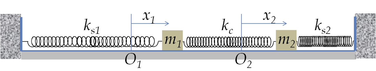
In a previous chapter on simple harmonic motion we studied oscillations of one block attached to a spring about its equilibrium. Wave phenomena arises as a result of the coupling of vibratory motions of many parts of a system. To develop a feel for the consequences of coupling of vibrations, we will study a simple system consisting of two blocks of masses \(m_1\) and \(m_2\) that are connected by a spring and supported on the two sides by two other springs as shown in Figure 14.7. In this section we will study this system analytically.
Subsection 14.2.1 (Calculus) Analytic Solution
We will study the one-dimensional motion of the coupled masses analytically by choosing the \(x\)-axis to coincide with the line of the springs and the blocks as shown in Figure 14.7. Let \(x_1\) and \(x_2\) be the displacements of the two blocks from their equilibrium positions. Note that \(x_1\) and \(x_2\) are not the \(x\)-coordinates of the blocks but rather the \(x\)-components of their displacements from the corresponding equilibrium positions.
Let \(k_{s1}\) be the spring constant of the spring connecting block \(m_1\) to the left support, \(k_{s2}\) the spring constant of the spring connecting block \(m_2\) to the right support, and \(k_c\) the spring constant of the spring coupling the two blocks as indicated in the figure.
The \(x\)-components of the equations of motion of the two blocks are
\begin{align}
\amp m_1\frac{d^2x_1}{dt^2} = -k_{s1} x_1-k_c (x_1-x_2),\tag{14.11}\\
\amp m_2\frac{d^2x_2}{dt^2} = -k_{s2} x_2+k_c (x_1-x_2).\tag{14.12}
\end{align}
Rather than solve these two equations for arbitrary values of the masses and constants, let us simplify the problem by looking at the case where masses are equal and two of the springs connecting the blocks to the support have equal spring constants.
\begin{align*}
\amp m_1 = m_2 \equiv m\\
\amp k_{s1} = k_{s2}\equiv k_s
\end{align*}
> Then, the equations of motion for \(x_1\) and \(x_2\) are
\begin{align}
\amp m\frac{d^2x_1}{dt^2} = -k_{s} x_1-k_c (x_1-x_2),\tag{14.13}\\
\amp m\frac{d^2x_2}{dt^2} = -k_{s} x_2+k_c (x_1-x_2).\tag{14.14}
\end{align}
To solve these equations, I will introduce new composite variables \(X\) and \(x\) in place of \(x_1\) and \(x_2\) by
\begin{align}
\amp X = \frac{x_1 + x_2}{2},\tag{14.15}\\
\amp x = x_1 - x_2.\tag{14.16}
\end{align}
Equations (14.13) and (14.14) then gives rise to the following equations of motion for \(X(t)\) and \(x(t)\text{.}\)
\begin{align}
\amp m\frac{d^2X}{dt^2} = -k_s X,\tag{14.17}\\
\amp m\frac{d^2x}{dt^2} = -\left( k_s+2k_c \right) x.\tag{14.18}
\end{align}
Equation (14.17) is an equation of motion of an oscillator of mass \(m\) and spring constant \(k_s\text{,}\) and Eq. (14.18) is an equation of motion of an oscillator of mass \(m\) and spring constant \(k_s+2k_c\text{.}\) Therefore, we can think of \(X\) and \(x\) as displacements of two fictitious simple harmonic oscillators of mass \(m\) attached to springs of spring constants \(k_s\) and \(\left( k_s+2k_c \right)\) respectively. The solution of these equations show that the variables \(X\) and \(x\) will oscillate with angular frequencies given by
\begin{align}
\amp \text{X oscillates at: }\ \ \ \omega_X = \sqrt{\frac{k_s}{m}}\tag{14.19}\\
\amp \text{x oscillates at: }\ \ \ \omega_x = \sqrt{\frac{k_s+2k_c}{m}}\tag{14.20}
\end{align}
The variables \(X\) and \(x\) are called normal modes and the angular frequencies \(\omega_X\) and \(\omega_x\) the normal frequencies of this system of two masses. The normal coordinates \(X\) and \(x\) execute simple harmonic motions of their corresponding frequencies and are given by
\begin{align}
\amp X(t) = A \cos(\omega_X t-\delta)\tag{14.21}\\
\amp x(t) = B \cos(\omega_x t-\phi)\tag{14.22}
\end{align}
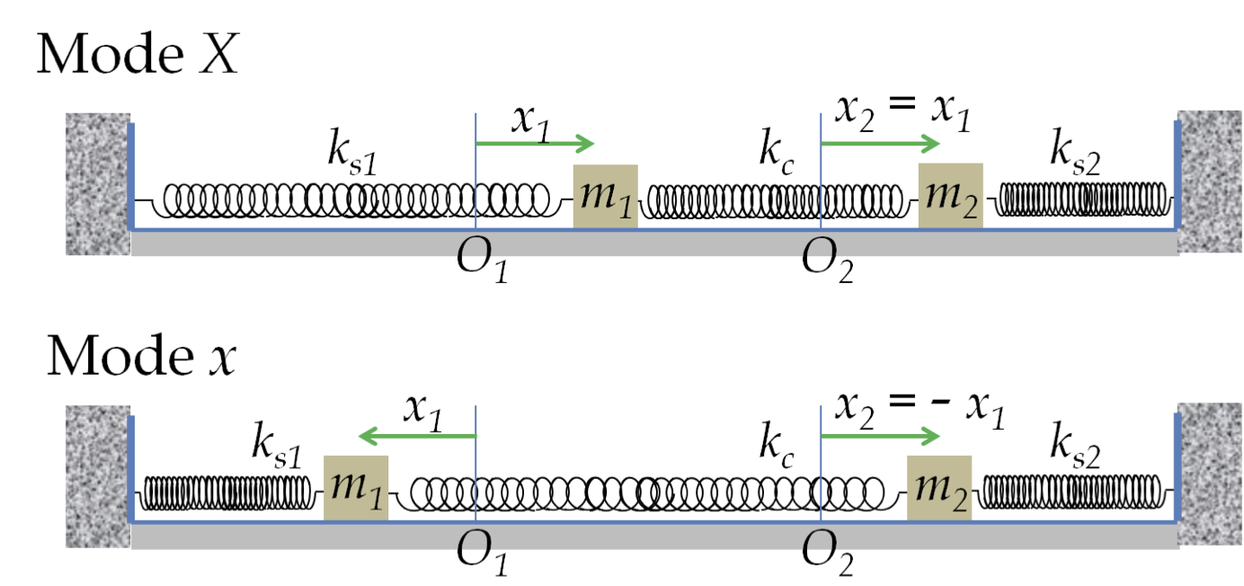
From Eqs. (14.15) and (14.16), we see that \(x=0\) when \(x_1=x_2\text{,}\) i.e., when the two blocks have equal displacment, the motion is that of mode \(X\text{.}\) When \(x_1=-x_2\text{,}\) i.e., ehen their displacments are opposite, \(X=0\text{,}\) in which case, the motion is in mode \(x\text{.}\) These are illustrated in Figure 14.8.