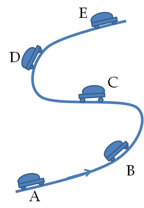
   
Logo image

Physics Bootcamp

Section 4.4 Acceleration

You know that you can make your car move from rest, speed up, slow down and bring to rest, or turn a corner. These are examples of changing velocity, either by changing magnitude or changing itd direction or both. The rate at which velocity, either speed or direction or both, changes is called acceleration.

Subsection 4.4.1 Average Acceleration

Suppose we are looking at what happens to velocity during an interval from \(t_i \) to \(t_ f \text{.}\) Let the instantaneous velocity (vector) at \(t_i \) be \(\vec v_i \) and at \(t_f \) be \(\vec v_f \text{.}\) Then, average acceleration is defined by
\begin{equation} \vec a_{\text{av}} = \dfrac{\vec v_f - \vec v_i}{t_f - t_i}.\tag{4.19} \end{equation}
We often use symbol \(\Delta \vec v\) to denote the change in velocity. Here,
\begin{equation} \Delta \vec v = \vec v_f - \vec v_i.\tag{4.20} \end{equation}
Writing the intertval of time as \(\Delta t\text{,}\) we write the definition of average acceleration more succinctly as
\begin{equation} \vec a_{\text{av}} = \dfrac{\Delta \vec v}{\Delta t}.\tag{4.21} \end{equation}
Since we are dividing a vector \(\Delta \vec v\) by a number \(\Delta t\text{,}\) average acceleration is also a vector. The direction of \(\vec a_{\text{av}}\) will be in the direction of change in velocity \(\Delta \vec v\text{.}\) In particular, the direction of acceleration has nothing to do with direction of velocity at any one instant, but instead with the change in velocity, i.e, how velocity of changing.
Figure 4.36 shows an object moving in a circle with constant speed of \(5\text{ m/s}\text{.}\) In (a), we see that the change in velocity between A and B points of the circle are neither in the direction of \(\vec v_A\) nor in the direction of \(\vec v_B\text{,}\) but its own direction as shown by vector \((\vec v_B - \vec v_A)\text{.}\) Since the change in velocity is not zero, the object’s average acceleration between A and B is not zero. In (b), another construction for change in velocity during B and C is shown. Try to draw for what happens between C and D and betwen D and A.
Figure 4.36. Changing velocity in a circular motion for an object with constant speed.
Just as with other vector quantities, we can analyze average acceleration in terms of its Cartesian components, \(a_{av,x} \text{,}\) \(a_{av,y} \text{,}\) and \(a_{av,z} \text{.}\) From these components, you can find the magnitude and direction of the acceleration vector.

Example 4.37.

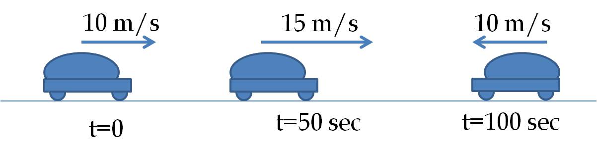
The velocity vectors of a car at three instants are shown in Figure 4.38. Use the arrow for the velocity at \(t=0\) for the scale for vectors in the figure. Use the geometric approach of vectors to find the average acceleration in the following intervals: (i) from \(t=0\) to \(t=50\) sec, (ii) from \(t=50\) sec to \(t=100\) sec, (iii) from \(t=0\) to \(t=100\) sec.
Figure 4.38.
Solution.
Figure 4.39 shows vector diagrams of the velocity vectors and the change in velocity for different intervals. The arrow for 10 m/s is taken as the scale for the drawing. The difference \(\vec v_2 - \vec v_1\) of two vectors is obtained by drawing the vector \(v_2\text{,}\) and then, drawing the vector \(\vec v_1\) at the tip of the vector \(\vec v_2\) with the direction of \(\vec v_1\) reversed. Then, the difference is equal to the vector from the tail of the vector \(\vec v_2\) to the tip of the reversed vector \(\vec v_1\text{.}\)
Figure 4.39.
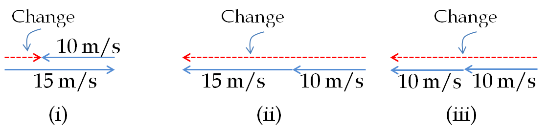
We find the following for the three intervals:
(i) For the interval from \(t=0\) to \(t=50\) sec, the change in velocity has magnitude 5 m/s and the direction towards the right in the figure. This change takes place over 50 sec. Therefore, the average acceleration in this interval has the magnitude \(0.1\, \text{m/s}^2\) and the direction towards the right.
(ii) For the interval from \(t=50\) sec to \(t=100\) sec, the change in velocity has magnitude 25 m/s and the direction towards the left in the figure. This change takes place over 50 sec. Therefore, the average acceleration in this interval has the magnitude \(0.5\, \text{m/s}^2\) and the direction towards the left.
(iii) For the interval from \(t=0\) sec to \(t=50\) sec, the change in velocity has magnitude 20 m/s and the direction towards the left in the figure. This change takes place over 100 sec. Therefore, the average acceleration in this interval has the magnitude \(0.2\, \text{m/s}^2\) and the direction towards the left.

Example 4.40. Average Acceleration.

The velocity of a car changes from \((v_x, v_y) = (5, 10) \) in m/s at time instant \(t=3.0 \) sec to \((5, -10) \) in m/s at instant \(t=8.0 \) sec.
(a) What are \(a_x \) and \(a_y \) of the average acceleration vector?
(b) What are the magnitude and direction of the average acceleration vector?
Answer.
(a) \((0, -4\text{ m/s}^2) \text{,}\) (b) \(4\text{ m/s}^2 \text{,}\) pointed towards the negative \(y \) axis.
Solution 1. a
Using the definition of the average velocity in components we get \(a_{av, x} = \dfrac{\Delta v_x}{\Delta t}\text{,}\) and similarly for other components.
\begin{align*} \amp a_{av,x} = \dfrac{5-5}{8-3}= 0,\\ \amp a_{av,y} = \dfrac{-10-10}{8-3}= -4\text{ m/s}^2. \end{align*}
Solution 2. b
From \(a_x \) and \(a_y \text{,}\) it is immediately clear that the acceleration vector has magnitude \(4\text{ m/s}^2 \) and pointed towards negative \(y \) axis.

Example 4.41. Acceleration as a Vector on an Incline.

A car stalls on a slippery road that is sloped at \(15^{\circ} \text{.}\) The car then slides down the road with an acceleration of \(2.5 \text{ m/s}^2\text{.}\)
(a) Suppose, your coordinates system has \(x \) axis horizontal and \(y \) axis vertically up. What will be \(x \) and \(y \) components of the acceleration vector \(\vec a \text{?}\)
Figure 4.42.
(b) Suppose your \(x \) axis is pointed down the road and \(y \) axis is vertical to the road. What will be \(x \) and \(y \) components of the acceleration vector \(\vec a \text{?}\)
Figure 4.43.
Answer.
(a) \((-2.41\text{ m/s}^2 \text{,}\) \(-0.65\text{ m/s}^2) \) or \((2.41\text{ m/s}^2 \text{,}\) \(-0.65\text{ m/s}^2) \text{,}\) (b) \((2.5\text{ m/s}^2 \text{,}\) \(0) \)
Solution 1. a
It is always a good idea to sketch the vector on a coordinate system where the tail of the vector is at the origin. This gives us a good idea of positive and negative values for the components. In Figure 4.44(a) below, we will find that both components are negative. If you draw the figure differently, as in (b), you might find the signs to come out differently.
Figure 4.44. For Example 4.41 (a).
Let \(a \) be the magnitude of the acceleration. Using trig in Figure 4.44(a), we find \(a_x = - a \cos\, 15^{\circ}\)\(=-2.41\text{ m/s}\text{,}\) and \(a_x = - a \sin\, 15^{\circ}\)\(=-0.65\text{ m/s}\text{.}\) Using Fig. (b), we get the sign of \(a_x \) changed to positive now.
This exercise illustrates that, although the physical description of acceleration, namely, \(2.5 \text{ m/s}^2\) down the slope is unique, the components depend upon how you draw the physical situation and the coordinates. This point is further explored in part (b) of this problem.
Solution 2. b
The axes are now completely different from the axes in part (a). Now, we do not get any projections on the \(y \) axis. Therefore, \(a_y = 0\text{.}\) From Figure 4.45, it is clear that \(a_x = a = 2.5\text{ m/s}^2\text{.}\)
Figure 4.45. Figures for Example 4.41(b).

Checkpoint 4.46. Acceleration of a Car Moving at Constant Speed on a Curved Road.

A car is moving at a constant speed of \(5\) m/s on a curved road as shown in Figure 4.47. Suppose the time interval between successive points A, B, C, D, and E is \(30\) sec. (a) Draw the velocity vectors to scale at points A, B, C, D, and E. State the scale for your drawings.
(b) Find the average acceleration between successive points marked on the trajectory. Give both the magnitude and the direction.
Figure 4.47.

Subsection 4.4.2 Instantaneous Acceleration - Formal Definition

Average acceleration defined above does not tell us about moment-by-moment acceleration. For that Isaac Newton, introduced the concept of instantaneous acceleration, or more siply acceleration, based on concepts of limit and infinitesimal intervals, as we have done for instantaneous velocity.
If you find average acceleration using Eq. (4.21) for different interval values, i.e., different values of \(\Delta t\text{,}\) you will find that you get different velocities as was illustrated for a circular motion. Newton noticed that, when \(\Delta t\) becomes increasingly small, the differences in average acceleration so-obtained become less and less in a well-defined way such that it is possible to define a unique acceleration in the limit \(\Delta t\rightarrow 0\text{.}\) Denoting the instantaneous acceleration vector by \(\vec a \) and instantaneous velocity vector as \(\vec v\) we can write the definition of instantaneous velocity formally by
\begin{equation} \vec a = \lim_{\Delta t \rightarrow 0} \dfrac{\vec v\left(\text{at } (t+\Delta t)\right) - \vec v\left(\text{at } t\right)}{\Delta t} \equiv \frac{d\vec r}{dt}.\tag{4.22} \end{equation}
Unlike the magnitude of instantaneous velocity, which is called speed, the magnitude of instantaneous acceleration does not have any special name.
Eq. (4.22) is an abstract definition, which we can make more accessibale by looking at the components. Denoting \(\vec v\left(\text{at } (t+\Delta t)\right) - \vec v\left(\text{at } t\right)\) by \(\Delta \vec v \equiv (\Delta v_x, \Delta v_y, \Delta v_z)\text{.}\)
\begin{align*} \amp a_x= \lim_{\Delta t \rightarrow 0}\dfrac{\Delta v_x}{\Delta t} \equiv \frac{dv_x}{dt},\\ \amp a_y= \lim_{\Delta t \rightarrow 0}\dfrac{\Delta v_y}{\Delta t} \equiv \frac{dv_y}{dt},\\ \amp a_z= \lim_{\Delta t \rightarrow 0}\dfrac{\Delta v_z}{\Delta t} \equiv \frac{dv_z}{dt}. \end{align*}
These components of acceleration are also called \(x\)-, \(y\)-, and \(z\)-accelerations respectively. In a previous chapter, we have studied one-dimensional motion, where only one of them was non-zero. For general motion, you can expect all of them to be nonzero and you would need to keep track of them all.

Subsection 4.4.3 Acceleration from Slopes of \((v_x,\ v_y,\ v_z) \) vs \(t \) Plots.

Acceleration at an instant, also called the instantaneous acceleration, is the rate at which velocity is changing with time. In one-dimensional situation, we analyzed by only \(x\) component of acceleration for motion along \(x\)-axis. Analytically, this was given by the derivative of \(v_x\text{,}\) the \(x\)-component of velocity.
\begin{equation*} a_x = \dfrac{dv_x}{dt}. \end{equation*}
Since derivate of a function also equals slope of a graph of that function, we had used \(v_x\) versus \(t\) plot to find \(a_x\) when using graphical method.
\begin{equation*} a_x= \text{Slope of tangent to } v_x \text{ versus } t \text{ plot}. \end{equation*}
Now, with acceleration possible along arbitrary directions, we can choose to analyze using all three Cartesian directions and calculate derivatives from the slopes of appropriate plots. Thus,
\begin{align*} \amp a_x= \text{Slope of tangent to } v_x \text{ versus } t \text{ plot}.\\ \amp a_y= \text{Slope of tangent to } v_y \text{ versus } t \text{ plot}.\\ \amp a_z = \text{Slope of tangent to } v_z \text{ versus } t \text{ plot}. \end{align*}
Once we have obtained \((a_x,\ a_y,\ a_z)\text{,}\) we can deduce the magnitude and direction of the acceleration vector as usual. For instance, magnitude of acceleration will be
\begin{equation} a = \sqrt{a_x^2 + a_y^2 + a_z^2},\tag{4.23} \end{equation}
and the direction will be given by one angle if the motion is 2-dimensional or by two angles if the motion is 3-dimensional.

Example 4.48. Acceleration from Slopes of Velocity Components.

The following figure shows plots of the \(x \) and \(y \) components of velocity, \(v_x \) and \(v_y \text{.}\) Find the acceleration in the component form at the following instants: (a) \(t = 1\text{ s}\text{,}\) (b) \(t = 3\text{ s}\text{,}\) (c) \(t = 5\text{ s}\text{,}\) (d) \(t = 7\text{ s}\text{,}\) (e) \(t = 9\text{ s}\text{.}\)
Answer.
(a) \((0, 1\text{ m/s}^2)\text{,}\) (b) \((0, -2\text{ m/s}^2)\text{,}\) (c) \((-1\text{ m/s}^2, 1\text{ m/s}^2)\text{,}\) (d) \((-1\text{ m/s}^2, 1\text{ m/s}^2)\text{,}\) (e) \((0, 0)\text{.}\)
Solution.
We need to find slopes at the indicated instants by \(a_x = \dfrac{\Delta v_x}{\Delta t}\) and similarly for \(a_y\text{.}\)
\begin{align*} \amp \text{(a)}\ \ a_x = 0,\ \ a_y = 1\text{ m/s}^2,\\ \amp \text{(b)}\ \ a_x = 0,\ \ a_y = -2\text{ m/s}^2,\\ \amp \text{(c)}\ \ a_x = -1\text{ m/s}^2,\ \ a_y = 1\text{ m/s}^2,\\ \amp \text{(d)}\ \ a_x = -1\text{ m/s}^2,\ \ a_y = 1\text{ m/s}^2,\\ \amp \text{(d)}\ \ a_x = 0,\ \ a_y = 0, \end{align*}

Subsection 4.4.4 (Calculus) Instantaneous Acceleration

To obtain acceleration at a particular instant \(t \text{,}\) we seek average acceleration in an infinitesimal interval near the instant \(t \text{.}\) This leads to the ratio in Eq. (4.21) becoming a derivative.
\begin{equation} \vec a = \dfrac{d \vec v}{dt}.\tag{4.24} \end{equation}
We can express the Cartesian components of acceleration as derivatives of the corresponding Cartesian components of the velocity vector.
\begin{align} \amp a_x = \dfrac{dv_x}{dt}\tag{4.25}\\ \amp a_y = \dfrac{dv_y}{dt}\tag{4.26}\\ \amp a_z = \dfrac{dv_z}{dt}\tag{4.27} \end{align}
Since \(v_x = dx/dt \text{,}\) \(v_y = dy/dt \text{,}\) snd \(v_z = dz/dt \text{,}\) we find that we can express components of acceleration as second derivatives of the position.
\begin{align} \amp a_x = \dfrac{d^2x}{dt^2}\tag{4.28}\\ \amp a_y = \dfrac{d^2y}{dt^2}\tag{4.29}\\ \amp a_z = \dfrac{d^2z}{dt^2}\tag{4.30} \end{align}
This is often written compactly as
\begin{equation} \vec a = \dfrac{d^2\vec r}{dt^2}.\tag{4.31} \end{equation}

Example 4.49. Velocity and Acceleration from Position as Function of Time.

A car moves on a straight road such that its position from a reference point is given as \(x(t) = 3 + 5 t + 2 t^2 + 0.4 t^3,\ y=0,\ z=0\text{,}\) where \(t\) is in sec and \(x\) in meter. (a) Determine the velocity and acceleration at (i) \(t =0\text{,}\) (ii) \(t = 0.5\ \textrm{sec}\) and (iii) \(t = 1\ \textrm{sec}\text{.}\) (b) Determine the average velocity and average acceleration between \(t = 0\) and \(t = 1\ \textrm{sec}\text{.}\)
Solution 1. a
Taking time derivative of \(x\) successively, we get \(v_x\) and \(a_x\text{.}\)
\begin{align*} \amp v_x = 5 + 4t+1.2 t^2;\ v_y = 0;\ v_z = 0\ \ \Longrightarrow \vec v = (5 + 4t+1.2 t^2)\ \hat u_x\ \ \textrm{[Unit: m/s]}\\ \amp a_x = 4+2.4 t;\ a_y = 0;\ a_z = 0\ \ \Longrightarrow \vec a = (4+2.4 t)\ \hat u_x\ \ \textrm{[Unit: m/s}^2\text{]} \end{align*}
Put the values of \(t\) for the instants in question. For instance, when you put (iii) \(t=1\) you get
\begin{equation*} v_x = 10.2\,\text{m/s},\ \ a_x = 6.4\,\text{m/s}^2. \end{equation*}
Solution 2. b
The \(x\)-components of average velocity and average acceleration between \(t=0\) and \(t=1\) s are
\begin{align*} \amp v_{av,x} = \frac{x(1\ \textrm{s})-x(0)}{1\ \textrm{s}-0} = \frac{10.4\ \textrm{m} - 3\ \textrm{m}}{1\ \textrm{s}} = 7.4\ \textrm{m/s}\\ \amp a_{av,x} = \frac{v_x(1\ \textrm{s})-v_x(0)}{1\ \textrm{s}-0} = \frac{10.2\ \textrm{m/s} - 5\ \textrm{m/s}}{1\ \textrm{s}} = 5.2\ \textrm{m/s}^2 \end{align*}
Since the \(y\)- and \(z\)-components are zero here, the magnitudes of the average velocity and average acceleration are equal to the absolute value of their \(x\)-components, and since the \(x\)-components are positive, the directions of these physical quantities are towards the positive \(x\)-axis.

Example 4.50. (Calculus) Acceleration of an Airplane during a Takeoff.

The velocity of an airplane during the takeoff is given in the component form with respect to some coordinate system: \(\vec v = (10\, t, 0, 3\, t^2) \) in m/s units with \(t \) is in seconds. Note the value of \(t \) is restricted to the time during the takeoff, which we will take to be \(0 \lt t \lt 10 \) in seconds.
(a) What is the acceleration of the plane at an arbitray instant \(t \) in \((0, 10) \) sec interval?
(b) What is the acceleration at \(t=2 \) sec?
(c) What are the components of the average acceleration during this time interval? Note this will not be a function of \(t \text{.}\)
NOTE: Time average of a function between instants \(t_1\) and \(t_2\) is defined by
\begin{equation*} f_{av} = \dfrac{1}{t_2-t_1}\, \int_{t_1}^{t2}\, f(t) dt. \end{equation*}
Answer.
(a) \((10,\ 0,\ 6\, t)\) in units of \(m/s^2\) if \(t\) is in sec. (b) \((10\text{ m/s}^2,\ 0,\ 12\text{ m/s}^2) \) , (c) \(\left(10\text{ m/s}^2,\ 0,\ 30\text{ m/s}^2 \right)\text{.}\)
Solution 1. a
Taking the derivative of \(\vec v \) we get
\begin{equation*} \vec a = (10, 0, 6\, t) \end{equation*}
in units of \(m/s^2\) if \(t \) is in seconds.
Solution 2. b
Putting \(t = 2 \) in the answer in (a) gives us the acceleration at \(t = 2\text{ sec} \text{.}\)
\begin{equation*} \vec a = (10, 0, 12). \end{equation*}
Solution 3. c
For average acceleration, we will average the time-dependent acceleration with respect to time. Time-average of a function \(f(t)\) between \(t=t_1 \) and \(t=t_2\) is defined by
\begin{equation*} f_{av} = \dfrac{1}{t_2-t_1}\, \int_{t_1}^{t2}\, f(t) dt. \end{equation*}
We need to do this only for the \(a_z \) since that is the only part that is time-dependent.
\begin{equation*} a_{av,z} = \dfrac{1}{10}\,\int_0^{10}\, 6\,t\, dt = 30\text{ m/s}^2. \end{equation*}
Therefore,
\begin{equation*} \vec a_{av} = \left(10\text{ m/s}^2,\ 0,\ 30\text{ m/s}^2 \right). \end{equation*}

Exercises 4.4.5 Exercises

1. Velocity and Acceleration of a Projectile from Position as Function of Time.

The position of a projectile in the air is monitored with respect to a reference point in a Cartesian coordinate system. The \(x\)-axis of the Cartesian coordinate system is in the horizontal direction and the \(y\)-axis vertically up. The \(z\)-coordinate of the projectile does not change with time. The data for the \(x\) and \(y\)-coordinates are plotted and the following functions fit the \(x\) vs \(t\) and \(y\) vs \(t\) curves: \(x(t) = 40 t\) and \(y(t) = 60 t - 5 t^2\text{.}\) (a) Find the instantaneous velocity of the projectile at the following instants: (i) \(t=0\text{,}\) (ii) \(t=4\ \textrm{sec}\text{,}\) (iii) \(t=8\ \textrm{sec}\text{,}\) and (iv) \(t=10\ sec\text{.}\) (b) Find the instantaneous acceleration of the projectile at the following instants: (i) \(t=0\text{,}\) (ii) \(t=4\ \textrm{sec}\text{,}\) (iii) \(t=8\ \textrm{sec}\text{,}\) and (iv) \(t=10\ \textrm{sec}\text{.}\)
Solution 1. a
Calculating the derivatives we find
\begin{align*} \amp v_x = 40;\ v_y = 60 - 10 t;\ v_z = 0\ \ \Longrightarrow \vec v = 40\ \hat u_x + (60 - 10 t)\ \hat u_y\ \ [\textrm{m/s}]\\ \amp a_x = 0;\ a_y = - 10 ;\ v_z = 0\ \ \Longrightarrow \vec a = - 10 \ \hat u_y\ \ [\textrm{m/s}^2] \end{align*}
Plug in the values of \(t\) for the components of the instantaneous velocity and acceleration at particular instants. The magnitudes and directions of the velocity and acceleration can be obtained in the usual way.
(i) \(v_x(0) = 40\ \textrm{m/s}\text{,}\) \(v_y(0) = 60\ \textrm{m/s}\text{,}\)\(\ v_z(0) = 0\text{,}\)
\begin{equation*} v(0) = \sqrt{(40\ \textrm{m/s})^2 + (60\ \textrm{m/s})^2} = 72\ \textrm{m/s}, \end{equation*}
\begin{equation*} \theta = \tan^{-1}\left(\frac{60\ \textrm{m/s}}{40\ \textrm{m/s}} \right)=56^{\circ}. \end{equation*}
(ii) \(v_x(4) = 40\ \textrm{m/s}\text{,}\) \(v_y(4) = 20\ \textrm{m/s}\text{,}\) \(v_z(4) = 0\text{,}\) \(v(4) = 45\ \textrm{m/s}\text{,}\) \(\theta = 27^{\circ}\text{.}\)
(iii) \(v_x(8) = 40\ \textrm{m/s}\text{,}\) \(v_y(8) = -20\ \textrm{m/s}\text{,}\) \(v_z(8) = 0\text{,}\) \(v(8) = 45\ \textrm{m/s}\text{,}\) \(\theta = 333^{\circ}\text{.}\)
(iv) \(v_x(10) = 40\ \textrm{m/s}\text{,}\) \(v_y(10) = -40\ \textrm{m/s}\text{,}\) \(v_z(10) = 0\text{,}\) \(v(8) = 72\ \textrm{m/s}\text{,}\) \(\theta = 315^{\circ}\text{.}\)
Solution 2. b
The instantaneous accelerations are computed in a similar way as (a).

2. Velocity and Acceleration of a Car Moving in a Circular Track from Position.

A car moves on a circular track. A coordinate system is chosen whose origin coincides with the center of the circle and the circle falls in the \(xy\)-plane. The position of the car with time varies according to the following functions of time: \(x(t) = 2 \cos\left(\frac{\pi}{100} t\right)\text{,}\) \(y(t) = 2 \sin\left(\frac{\pi}{100} t\right)\text{,}\) \(z=0\text{.}\) Determine the velocity and acceleration of the car at (i) \(t =0\text{,}\) (ii) \(t = 50\ \textrm{sec}\text{,}\) (iii) \(t = 100\ \textrm{sec}\text{,}\) (iii) \(t=150\ \textrm{sec}\text{,}\) and (iv) \(t=200\ \textrm{sec}\text{.}\)
Solution.
In this solution I will give only the components of the vectors and you can practice in constructing the magnitude and direction. The general formula for the components of the velocity and acceleration obtained by performing the time derivatives are
\begin{align*} \amp v_x = -2\frac{\pi}{100}\sin\left(\frac{\pi}{100}\ t \right);\ v_y = 2\frac{\pi}{100}\cos\left(\frac{\pi}{100}\ t \right);\ v_z = 0\ \ \textrm{[Unit: m/s]};\\ \amp a_x = -2\left(\frac{\pi}{100}\right)^2\cos\left(\frac{\pi}{100}\ t \right) \ \ [\textrm{Unit: m/s}^2]\\ \amp a_y = -2\left(\frac{\pi}{100}\right)^2\sin\left(\frac{\pi}{100}\ t \right) ;\ a_z = 0\ \ [\textrm{Unit: m/s}^2] \end{align*}
The instantaneous values at particular instants are obtained by substituting the value of \(t\text{.}\) For instance, at \(t=0\text{,}\) we find that \(v_x = 0\text{,}\) \(v_y = 2\pi/100\ \textrm{m/s}\text{,}\) \(v_z = 0\text{,}\) \(a_x = -2\left( \pi/100\right)^2\) m/s\(^2\text{,}\) \(a_y = 0\text{,}\) and \(a_z = 0\text{.}\)