   
Logo image

Physics Bootcamp

Section 30.6 Gauss’s Law Bootcamp

Exercises Exercises

Electric Field Flux

1. Electric Flux of Constant Electric Field for Various Orientation of the Area.
Follow the link: Example 30.6.
2. (Calculus) (Calculus) Electric Flux of a Point Charge Through a Spherical Surface.
Follow the link: Example 30.9.
3. Electric Flux Through a Disk Above a Point Charge.
Follow the link: Example 30.10.

Gauss’s Law

4. Using Gauss’s Law To Find Electric Flux Through Closed Surfaces From Charges.
Follow the link: Example 30.14.
5. Electric Field of Charged Thick Concentric Spherical Shells.
Follow the link: Example 30.17.
6. Electric Field of Two Oppositely Charged Thin Spherical Shells.
Follow the link: Example 30.18.
7. Flux of Electric Field of a Spherical Charge Distribution Through Various Surface and Meaning of Zero Flux.
Follow the link: Exercise 30.3.4.1.
8. Electric Flux of Charges on a Copper Spherical Ball.
Follow the link: Exercise 30.3.4.2.
9. Electric Flux and Electric Field of a Charged Copper Ball Surrounded by a Gold Spherical Shell.
Follow the link: Exercise 30.3.4.3.
10. Electric Field of a Non-Uniform Charge Distribution of Spherical Symmetry.
Follow the link: Exercise 30.3.4.4.
11. Detemining if a Charge Distribution has Approximate Cylindrical Symmetry.
Follow the link: Example 30.23.
12. Electric Field of a Charged Thin Long Wire.
Follow the link: Example 30.24.
13. Electric Field of a Uniformly Charged Cylindrical Shell.
Follow the link: Example 30.25.
14. Electric Field of Oppositely Charged Two Concentric Cylindrical Shells.
Follow the link: Exercise 30.4.4.1.
15. Electric Field of a Uniformly Charged Rod Surrounded by an Oppositely Charged Cylindrical Shell.
Follow the link: Exercise 30.4.4.2.
16. Surface Charge Density on a Uniformly Charged Sheet from Given Electric Flux.
Follow the link: Exercise 30.5.5.1.
17. Electric Flux Through Tilted Area from Electric Field of Two Oppositely Charged Plates.
Follow the link: Exercise 30.5.5.2.

Miscellaneous

18. Flux Through One Side of a Cube for Charge at the Center.
A point charge \(q\) is at the center of a cube of side \(a\text{.}\) Find the electric flux through one of its sides.
Hint.
Think how you can use Gauss’s law for closed surface.
Answer.
\(\dfrac{1}{6}\:\dfrac{q}{\epsilon_0}\text{.}\)
Solution.
By Gauss’s law, flux through a closed surface equals \(q_\text{enc}/\epsilon_0\text{.}\) Now, if we consider the surfaces of the cube making a closed surface around the charge at the center,we will have
\begin{equation*} \Phi_{\text{cube}} = \frac{q}{\epsilon_0}. \end{equation*}
Since the charge is at the center of the cube, we can assert that flux through each face of the cube will be same based on the symmetry.
\begin{equation*} \Phi_{\text{cube}} = 6\times \Phi_{\text{one face}}. \end{equation*}
Therefore, we will have
\begin{equation*} \Phi_{\text{one face}} = \dfrac{1}{6}\:\dfrac{q}{\epsilon_0}. \end{equation*}
19. Flux Through One Side of a Cube for Charge at One Corner.
A charge \(q\) is placed at one of the corners of a cube of side \(a\text{.}\) Find the electric flux through the shaded face shown in the figure. Assume \(q>0\text{.}\)
Hint.
Think of enclosing the charge symmetrically by a larger cube, and the, use Gauss’s law on the larger cube.
Answer.
\(\dfrac{1}{24}\:\dfrac{q}{\epsilon_0}\text{.}\)
Solution.
Since the charge is at one corner of the cube, we do not have a symmetry like the one we had when the charge was located at the center of the cube in Exercise 30.6.18.
However, we can imagine adding seven more cubes to form a larger cube of side \(2a\) so that the charge now sits at the center of the larger cube. According to Gauss’s law, the electric flux trough the surface of the larger cube will be
\begin{equation*} \Phi_{\text{larger cube}} = \dfrac{q}{\epsilon_0}. \end{equation*}
Now, there are \(8\) smaller cubes, each with \(3\) faces in the same symmetric situation. This makes net flux equal to \(8\times 3=24\) times the surface of the original face. Therefore, flux through the shaded face of the original cube will be
\begin{equation*} \Phi_{\text{larger cube}} = 24\times \Phi_{\text{shaded face original}}. \end{equation*}
Therefore, the flux through the shaded face of the original cube will be
\begin{equation*} \Phi_{\text{shaded face original}} = \dfrac{1}{24}\:\dfrac{q}{\epsilon_0}. \end{equation*}
20. Electric Field of Two Parallel Charged Wires.
Two non-conducting uniformly charged thin straight wires of line charge densities \(\lambda_1=\lambda_0\) and \(\lambda_2=-\lambda_0\) respectively are placed a distance \(2d\) apart as shown in Figure 30.33.
Suppose the wires are parallel to the \(z\) axis and cross the \(xy\)-plane on the \(x\) axis at \(x_1= -d\) and \(x_2= +d\text{,}\) respectively. Find electric field at a point P in the \(xy\)-plane. Numerical values to use: \(\lambda_0 = 10\ \mu\text{C/m}\text{,}\) \(d=1.0\text{ cm}\text{,}\) \(x = 2\text{ cm}\text{,}\) and \(y = 4\text{ cm}\text{.}\)
Figure 30.33. For Exercise 30.6.20.
Hint.
Use superposition of the electric field of the electric fields of the two wores. Pay attention to the directions.
Answer.
\(37,500\text{ N/C}\) at clockwise angle \(82^\circ\) from positive \(x\)-axis.
Solution.
I will work out the numerical problem.
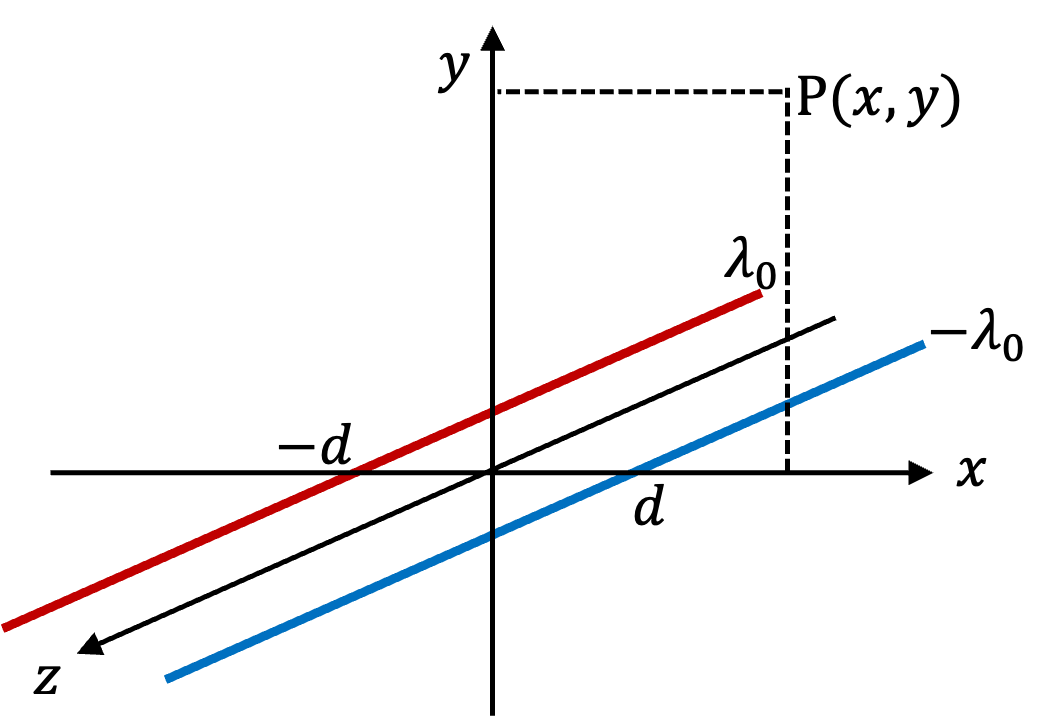
Let \(r_1\) and \(r_2\) be the distance from the wires to the field point \((x,y)\) in the \(xy\)-plane .
\begin{align*} r_1 \amp = \sqrt{(x+d)^2 + y^2}, \\ \amp = \sqrt{(2+1)^2 + 4^2} = 5\text{ cm}, \\ r_2 \amp = \sqrt{(x-d)^2 + y^2}, \\ \amp = \sqrt{(2-1)^2 + 4^2} = \sqrt{17}\text{ cm}. \end{align*}
Using the formulas for the magnitudes of the electric fields from charges on long wire, which is done by Gauss’s law for cyclindrical case, we get
\begin{align*} E_1 \amp = \dfrac{|\lambda_1|}{2\pi\epsilon_0}\,\dfrac{1}{r_1} \\ \amp = \dfrac{ 10\times 10^{-6}}{2\pi\times8.85\times 10^{-12}}\,\dfrac{1}{5} = 35,967\text{ N/C} \\ E_2 \amp = \dfrac{|\lambda_2|}{2\pi\epsilon_0}\,\dfrac{1}{r_2} \\ \amp = \dfrac{ 10\times 10^{-6}}{2\pi\times8.85\times 10^{-12}}\,\dfrac{1}{\sqrt{17}} = 67,972\text{ N/C} \end{align*}
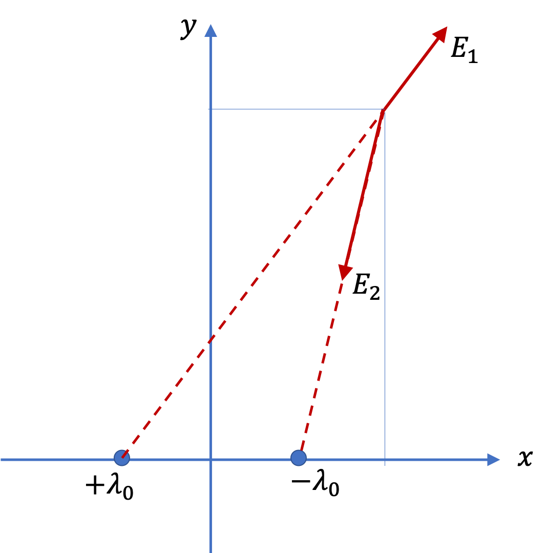
Now we need to add them vectorially. The net field is not just sum of the magnitudes, as you know from vector addition.
\begin{equation*} E_P \ne E_1 + E_2. \end{equation*}
We will first compute \(x\) and \(y\) components of the two fields so that we can find \(x\) and \(y\) components of the net field.
\begin{align*} E_{1x} \amp = E_1\, \dfrac{x+d}{r_1}, \\ \amp = 35,967\text{ N/C}\, \dfrac{3}{5} = 21,580\text{ N/C}, \\ E_{1y} \amp = E_1\, \dfrac{y}{r_1}, \\ \amp = 35,967\text{ N/C}\, \dfrac{4}{5} = 28,774\text{ N/C}. \end{align*}
Similarly, we work out the components of the field of wire 2. But, here we need to multiply by \(-1\) since we have a negative charge.
\begin{align*} E_{2x} \amp = E_2\, \dfrac{-(x-d)}{r_2}, \\ \amp = 67,972\text{ N/C}\, \dfrac{-1}{\sqrt{17}} = -16,486\text{ N/C}, \\ E_{2y} \amp = E_2\, \dfrac{-y}{r_2}, \\ \amp = 67,972\text{ N/C}\, \dfrac{-4}{\sqrt{17}} = -65,943\text{ N/C}. \end{align*}
Therefore, the components of the net field are
\begin{align*} E_x \amp = E_{1x} + E_{2x} = 21,580 -16,486 = 5,094\text{ N/C},\\ E_y \amp = E_{1y} + E_{2y} = 28,774 - 65,943 = -37,169\text{ N/C} \end{align*}
Therefore, the magnitude of the field is
\begin{equation*} E = \sqrt{ E_x^2 + E_y^2} = 37,500\text{ N/C}, \end{equation*}
and the direction can be given by clockwise angle from positive \(x\) axis.
\begin{equation*} \theta = \tan^{-1}\left( \dfrac{-37,169}{5,094} \right) = - 82^\circ. \end{equation*}
21. Electric Field at a Point Above a Hole in a Charged Sheet.
A disk of radius \(R\) is cut in a non-conducting large plate that is uniformly charged with charge density \(\sigma\) (coulomb per square meter). Find the electric field at a height \(h\) above the center of the disk. (\(h>>R\text{,}\) \(h\lt \lt l\) or \(w\)).
Hint.
Fill hole with \(\pm\sigma\) and then use superposition of plane of charge and a disk.
Answer.
\(\dfrac{\sigma h}{2\epsilon_0\,\sqrt{R^2+h^2}}\text{.}\)
Solution.
Imagine filling the hole with equal and opposite charge with charge densities \(+\sigma\) and \(-\sigma\text{.}\) When we include the small disk of charge \(+\sigma\) with the rest of the plane, we get one large plane of charge density \(+\sigma\text{.}\) The charge compensating disk of charge density \(-\sigma\) can be treated as a separate disk. The electric field at point P will be equal to the vector sum of the field of the entire plane and of the disk.
We know the formulas for the electric fields of large uniformly charged plate and of a uniformly charged disk. Here the field from the plane is pointed away from the plane and the field of the disk is towards the plane.
With \(z\) axis pointed up, the \(z\) components of electric fields from plate and disk are
\begin{align*} E_{\text{plate},z} \amp = \dfrac{\sigma}{2\epsilon_0},\\ E_{\text{disk},z} \amp = -\dfrac{\sigma}{2\epsilon_0}\: \left( 1-\dfrac{h}{\sqrt{R^2 + h^2}} \right). \end{align*}
Adding these components of fields we obtain the \(z\) component of the net electric field.
\begin{equation*} E_{z} = \dfrac{\sigma}{2\epsilon_0}\: \dfrac{h}{\sqrt{R^2 + h^2}} \end{equation*}
Since, the field has only \(z\) component, this also is the magnitude of the net electric field. The direction will be away from the plate if \(\sigma\gt 0\) and towards the plate if \(\sigma\lt 0\text{.}\)
22. Electric Field of a Charged Sphere with a Spherical Cavity.
A noncoducting sphere of radius \(R\) has uniform charge density \(\rho_0\text{.}\) A spherical cavity of radius \(\frac{R}{2}\) is then removed, resulting in the configuration shown in Figure 30.34. Find electric field at points (a) \(\text{P}_1\text{,}\) (b) \(\text{P}_2\text{,}\) (c) \(\text{P}_3\text{,}\) (d) \(\text{P}_4\text{,}\) and (e) \(\text{P}_5\text{.}\)
Figure 30.34. For Exercise 30.6.22.
Hint.
Think filling the cavity with opposite charges and restoring spherical symmetry.
Answer.
(a) \(\frac{\rho_0 R}{6\epsilon_0}\text{,}\) left, (b) \(\frac{\rho_0 R}{6\epsilon_0}\text{,}\) left, (c) \(\frac{\rho_0 R}{6\epsilon_0}\text{,}\) left, (d) \(\frac{17\rho_0 R}{54\epsilon_0}\text{,}\) right, (d) \(\frac{5\rho_0 R}{216\epsilon_0}\text{,}\) right, (e)
Solution.
As before in other problems with cavities, we will fill the cavity with opposite charges so that we can restore symmetries in charge distribution. Suppose, charge density \(\rho_0\) is positive, then we will fill the cavity with positive \(\rho_0\) and equal amout of negative \(-\rho_0\text{.}\) Then, we include \(\rho_0\) with the original charges.
Figure 30.35. For Exercise 30.6.22.
This process makes two spherically symmetric charge distributions. Since we already know expressions for electric field in uniformly charged sphere, we will just use those formulas when we superimpose the answers.
We will work out directions for \(\rho_0\gt 0\text{.}\) If \(\rho_0\lt 0\text{,}\) you wil ljust have to flip the arrow.
(a) At \(\text{P}_1\text{,}\) the field from smaller sphere will be to the right and field from the larger sphere will be to the left. This will mean they will subtract. The magnitudes of the two are such that both have contribution from all charges in their distributions since \(\text{P}_1\) is outside of both - at the edge will be taken as just outside. Hence, magnitude of the field there will be
\begin{equation*} E_1 = \frac{\rho_0 R}{3\epsilon_0} - \frac{\rho_0 R/2}{3\epsilon_0} = \frac{\rho_0 R}{6\epsilon_0}. \end{equation*}
The direction is to the left.
(b) At \(\text{P}_2\text{,}\) we have zero field from the smaller sphere. Since this point is an inside point for the larger sphere, we will use \(E_\text{in}\) formula for that.
\begin{equation*} E_2 = \frac{\rho_0 R/2}{3\epsilon_0} = \frac{\rho_0 R}{6\epsilon_0}. \end{equation*}
The direction is to the left.
(c) At \(\text{P}_3\text{,}\) we have zero field from the larger sphere. Since this point is an outside point for the smaller sphere, we will use \(E_\text{out}\) formula for that. At the edge of this sphere we get
\begin{equation*} E_3 = \frac{\rho_0 R}{6\epsilon_0}. \end{equation*}
The direction is to the left.
(d) \(\text{P}_4\) is outside of both spheres with larger one’s field pointed to the right and smaller one’s pointed left. From their superposition we get the magnitude
\begin{align*} E_4 \amp = \frac{\frac{4}{3}\pi R^3 \rho_0 }{4\pi R^2 \epsilon_0} - \frac{\frac{4}{3}\pi (R/2)^3 \rho_0 }{4\pi (3R/2)^2 \epsilon_0}\\ \amp = \frac{17}{54}\ \frac{\rho_0 R}{\epsilon_0}. \end{align*}
The direction is to the right.
(e) \(\text{P}_5\) is outside of both spheres with larger one’s field pointed to the right and smaller one’s pointed left. From their superposition we get the magnitude
\begin{align*} E_4 \amp = \frac{\frac{4}{3}\pi R^3 \rho_0 }{4\pi (3R/2)^2 \epsilon_0} - \frac{\frac{4}{3}\pi (R/2)^3 \rho_0 }{4\pi R^2 \epsilon_0}\\ \amp = \frac{5}{216}\ \frac{\rho_0 R}{\epsilon_0}. \end{align*}
The direction is to the right.
23. Electric Field at the Center of a Small Disk Removed From a Uniformly Charged Spherical Shell.
A spherical shell of radius \(R\) is charged uniformly with constant surface charge density \(\sigma_0\text{.}\) A small piece of the shell is then removed, resulting in a hole in the spherical shell. Suppose the removed part is almost flat circular disk of radius \(a\text{.}\) What is the electric field an infinitesimal distance \(d\) above the center of the hole so that you can asume \(d\lt lt a\text{?}\)
You might find magnitude of electric field of a disk of radius \(a\) and charge density \(\sigma\) at a distance \(d\) above the center to be
\begin{equation*} E = \frac{|\sigma|}{2\epsilon_0}\left( 1 - \frac{d}{\sqrt{d^2+a^2}}\right). \end{equation*}
For \(d\lt\lt a\text{,}\) this simplifies to \(\frac{|\sigma|}{2\epsilon_0}\text{.}\)
Hint.
Think filling the hole with opposite charges and restoring spherical symmetry with one and using the large sheet formula for the other.
Answer.
\(\sigma_0/2\epsilon_0\) radially out if \(\sigma_0\gt 0\text{.}\)
Solution.
As before in other problems with cavities, we will fill the cavity with opposite charges so that we can restore symmetries in charge distribution. Suppose, charge density \(\sigma_0\) is positive, then we will fill the cavity with positive \(\sigma_0\) and equal amout of negative \(-\sigma_0\text{.}\) Then, we include \(\sigma_0\) with the original charges. Then, electric field at P will be a vector sum of the electric field by the spherical shell and the disk as shown in Figure 30.36.
Figure 30.36. For Exercise 30.6.23.
Let us use a \(z\) axis to take care of directions. By Gauss’s law, we get electric field of the shell, which we will wrtie as \(z\) component at point P.
\begin{equation*} E_{\text{shell},z} = \frac{4\pi R^2 \sigma_0}{4\pi R^2 \epsilon_0} = \frac{\sigma_0}{\epsilon_0}. \end{equation*}
Since \(d \lt\lt a\text{,}\) the \(z\) component of the electric field from the negative charges on the disk will be
\begin{equation*} E_{\text{disk},z} = -\frac{\sigma_0}{2\epsilon_0}. \end{equation*}
Adding these two we get
\begin{equation*} E_z = \frac{\sigma_0}{2\epsilon_0}. \end{equation*}
Therefore, magnitude is \(\frac{\sigma_0}{2\epsilon_0}\) and direction is radially out from the center of the spherical shell.