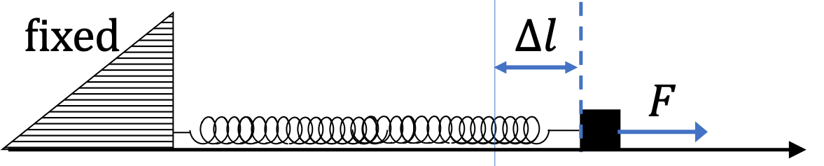
A \(30\text{-kg}\) box on a smooth floor is attached to a spring of spring constant \(100\text{ N/m}\) and pulled horizontally by an increasing force \(F \) until the point when the box starts to slide. At that instant, \(F = 75\text{ N}\text{.}\) The coefficient of static friction between the bottom of the box and the floor surface is \(0.2\text{.}\)
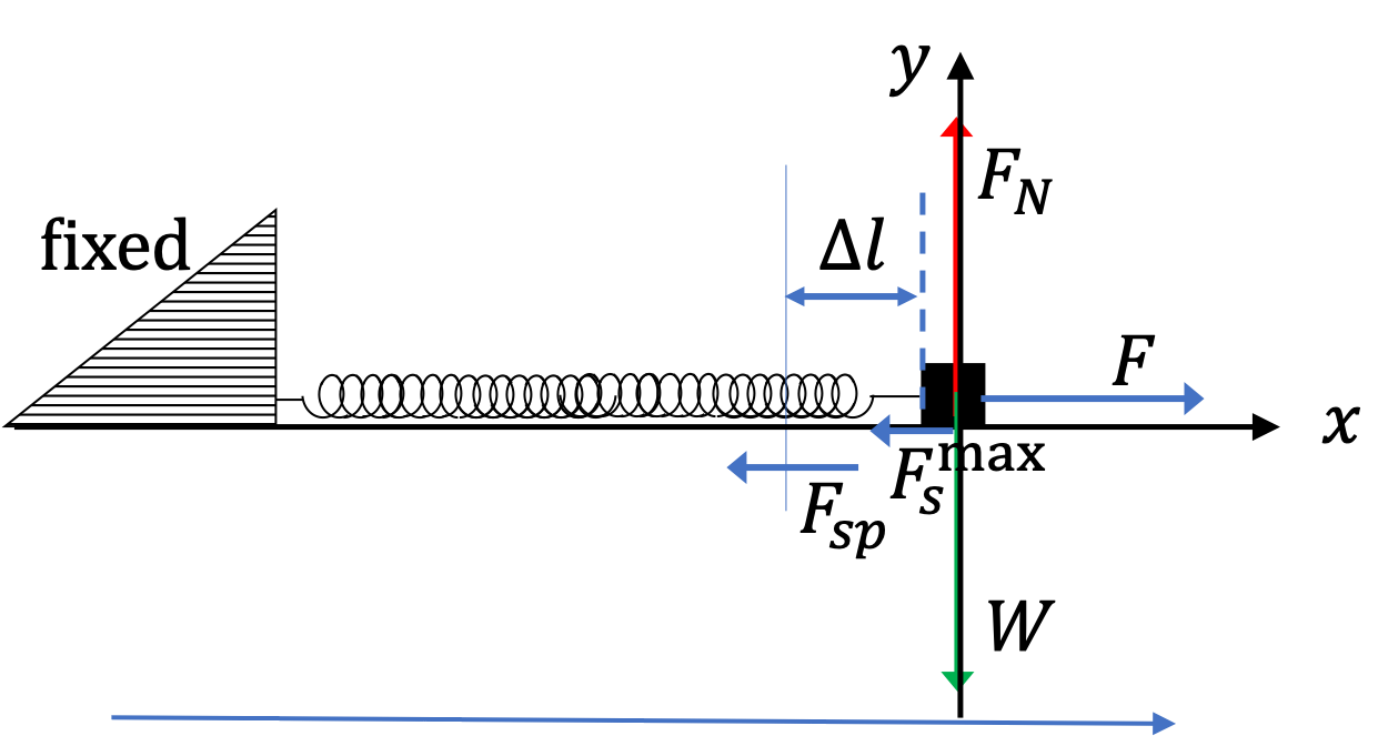
Since acceleration of the block is zero, forces on the block are balanced. Since every force is along one or the other axis, it is very easy to write equations of motion along the two axes directly. Lets also just use \(F_{s}^{\text{max}} = \mu_s F_N \text{.}\) Also, lets use \(F_{sp} = k \Delta l\text{.}\) We need to find \(\Delta l\text{.}\)
\begin{align*}
\amp F - \mu_s F_N - k\Delta l = 0, \\
\amp F_N - mg = 0,
\end{align*}
Solve the second equation for \(F_N \) and use that in the first equation, which we solve for \(\Delta l\text{.}\)
\begin{equation*}
\Delta l = \dfrac{1}{k} \left( F -\mu_smg \right).
\end{equation*}
Putting the numerical values in this equation we get
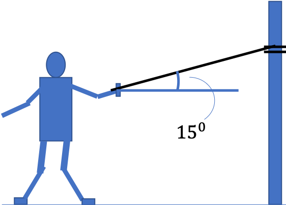
54.An Athlete Pulling on A Rope - Balancing Forces to Find Minimum \(\mu_s\).
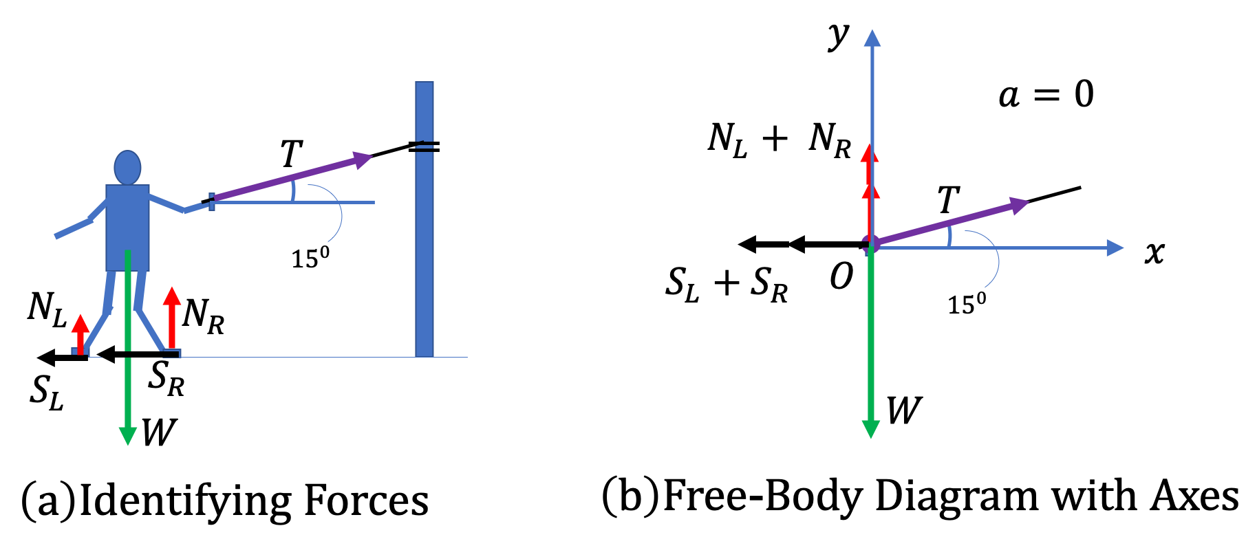
A \(100\text{-kg}\) athlete pulls a rope attached to a strong pole at an angle of \(15^{\circ}\) from horizontal such that the tension in the rope devlops to \(800\text{ N}\text{.}\)
(b) What must be minimum value of the coefficient of static friction between the sole of the shoes of the athlete and the floor so that the athlete does not slip on the floor while he is pulling on the rope?
We start by identifying forces on the block in Figure 6.140, where I have used symbols for the forces: \(W \) for weight, \(T \) for weight, \(N_L \) for the normal on the left foot, \(N_R \) for the normal on the right foot, \(S_L \) for the static friction on the left foot, and \(S_R \) for the static friction on the right foot.
In the translational motion, we can combine the normal forces into one and call that \(N=N_L+N_R\text{,}\) and similary for the static friction, \(S=S_L+S_R\text{.}\) We will have to keep them separate when we look at rotation.
Since acceleration of the block is zero, the forces are balanced. Since only \(T \) is not along one of the axes, we will need to work out its components. Let \(\theta \) stand for angle \(15^{\circ}\text{.}\)
Now, we can write the equations of motion along the two axes.
\begin{align*}
\amp T\,\cos\,\theta - S = 0, \\
\amp T\,\sin\,\theta + N - W = 0,
\end{align*}
Here, the values of \(T \text{,}\)\(\theta\text{,}\) and \(W=mg\text{,}\) are known. Therefore, we solve the first equation to get \(S \text{,}\) and the second one for \(N \text{.}\)
\begin{align*}
\amp S = T\,\cos\,\theta = 800 \times \cos\,15^{\circ} = 773\text{ N}, \\
\amp N = W - T\,\sin\,\theta = 100\times 9.81 - 800 \times \sin\,15^{\circ} = 774\text{ N}.
\end{align*}
From the problem description, we need the minimum \(\mu_s \text{.}\) That means, if we assume the \(S \) we found was the \(S^{\text{max}}\text{,}\) then the \(\mu_s \) we will get will be the minimum required for the static condition to hold.
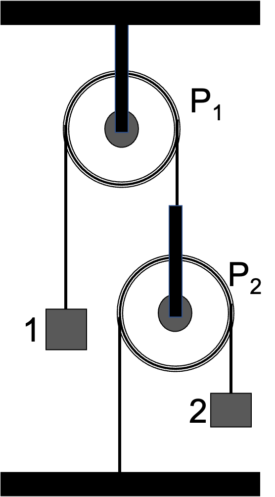
55.Motion of One Pulley and Two Blocks on One Pulley.
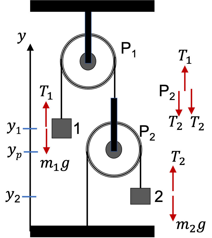
Figure 6.141 shows a two pulley two block system. While pulley \(\text{P}_1\) only rotates with its center remaining fixed, \(\text{P}_2\) rotates as well as moves. Assume both pulleys to be ideal (massless and frictionless) so that tension on the two sides of each pulley have the same magnitude. Do not assume tensions in the two strings are equal but you can assume that the length of strings do not change during the motion. Find the tensions in the two strings and accelerations of the two blocks.
Use an upward pointed \(y\) axis and write lengths of the two strings in terms of the \(y\) coordinates. From there deduce relation among accelerations of the two blocks.
Let us use upward pointed \(y\) axis as in Figure 6.142 to analyze the motion. Let \(y_1\text{,}\)\(y_p\text{,}\)\(y_2\) denote the positions of the centers of block 1, pulley \(P_2\text{,}\) and block 2 respectively. We will need \(y_p\) to figure out the relation between changes in \(y_1\) and \(y_2\text{.}\)
Let us look at each string to find relations among changes in these \(y\)’s. To facilitate this, let \(y_\text{top}\) be the \(y\) of the fixed pulley. Let us also denote lengths of the strings by \(l_1\) and \(l_2\) respectively. Then, we have
This relation between the accelerations and \(y\) equations of motion of the two blocks and the moving pulley (zero mass) will be sufficient to answer the questions about accelerations of the two blocks and the tensions. Using the force diagrams of each block we have the following equations.
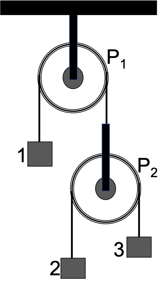
56.Practice with a Friend: Motion of One Pulley and Three Blocks on One Pulley.
Figure 6.143 shows a two pulley three block system. While pulley \(\text{P}_1\) only rotates with its center remaining fixed, \(\text{P}_2\) rotates as well as moves. Assume both pulleys to be ideal (massless and frictionless) so that tension on the two sides of each pulley have the same magnitude. Do not assume tensions in the two strings are equal but you can assume that the length of strings do not change during the motion. Find the tensions in the two strings and accelerations of the three blocks.
57.Movement of Three Blocks on Three Pulleys one of Which is Also Moving.
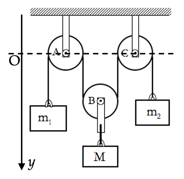
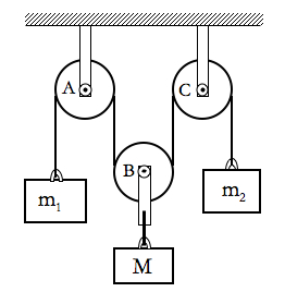
Three masses are connected to two fixed pulleys and a moving pulley as shown in the figure. Assume all pulleys massless and frictionless and all strings massless. Find the accelerations of the three masses.
To work out the constraint in the motion of the coupled system of masses and pulleys, let us work with a coordinate system with the origin at the level of the line joining A and C and the direction of the positive \(y\)-axis pointed down as shown in Figure 6.145. Let the \(y\)-coordinates of \(m_1\text{,}\)\(m_2\text{,}\)\(M\text{,}\) and B be \(y_1\text{,}\)\(y_2\text{,}\)\(y_3\text{,}\) and \(y_p\) respectively.
There are two constraints, namely the length of the string over the pulleys is constant and the distance between M and B is fixed. These physical constraints becomes
\begin{align*}
\amp y_1 +\pi R + y_p+\pi R +y_p + \pi R + y_3 = \textrm{constant}.\\
\amp y_3 - y_p = \textrm{constant}.
\end{align*}
By taking successive derivatives with respect to time, we get the following constraints among the \(y\)-components of the velocities and accelerations.
With the positive \(y\)-axis pointed down, we obtain the following \(y\)-components of the equations of motion for \(m_1\text{,}\)\(m_2\text{,}\) and the system constaining the mass \(M\) and the center pulley.
\begin{align}
\amp m_1 g - T = m_1 a_{1y}.\tag{6.81}\\
\amp m_2 g - T = m_2 a_{2y}.\tag{6.82}\\
\amp Mg - 2T = M a_{3y}.\tag{6.83}
\end{align}
To make use of Eq. (6.80), divide each equation here by masses.
\begin{align}
\amp g - \frac{1}{m_1} T = a_{1y}.\tag{6.84}\\
\amp g - \frac{1}{m_2} T = a_{2y}.\tag{6.85}\\
\amp g - \frac{2}{M} T = a_{3y}.\tag{6.86}
\end{align}
Multiply the last equation by 2 and add the three equations allows us to use Eq. (6.80) to arrive at
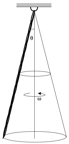
58.Rope Swinging in a Conical Path at Constant Speed.
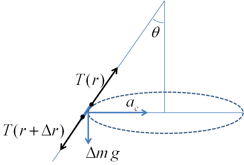
A rope of mass \(M\) and length \(L\) is swung uniformly with the angular speed \(\omega\) in a circle that makes an angle \(\theta\) with the vertical as shown in Figure 6.146 . What is the tension in the rope at a distance \(b\) from the top? Note: each element of the rope moves in a horizontal circle with uniform circular motion.
Consider a small element of the rope between \(r\) and \(r+\Delta r\) from the suspension point. This element of mass \(\Delta m = (M/L)\Delta r\) will be moving in a circle of radius \(R = r \sin\theta\) at the speed \(v = \omega r\text{.}\)
The free-body diagram of the forces on the element shows that there are three forces on it: the weight \(\Delta m g\) vertically down, the tension at \(r\) pulling the element towards the suspension point and the tension at \(r+\Delta r\) pulling the element away from the suspension. The acceleration of the element is pointed horizontally towards the center of the circle of motion.
and we arrive at the following rule for the rate of the change of the tension along the rope.
\begin{equation*}
\frac{dT}{dr} = - \frac{M \omega^2}{L} \ r.
\end{equation*}
To find the tension we need to integrate this equation. We have seen this type of equation when the velocity was a linearly increasing function of time and we needed the displacement. Similar technique can be used here. We notice that \(r=L\) corresponds to the free end of the rope at the end and the tension there will be zero. Therefore, let us integrate from \(r=L\) to \(r=r\) corresponding to \(T=0\) to \(T=T(r)\text{.}\)