Simple harmonic motion appears in a wide variety of physical settings. The defining characteristic of a system exhibiting a simple harmonic motion in some variable \(x\) is that second derivative of the variable is prportional to the negative of \(x\text{.}\)
\begin{equation*}
\frac{d^2x}{dt^2} = - \omega^2 x.
\end{equation*}
Variable \(x\) does not have to be \(x\)-coordinate. It can be some angle, e.g., in a simple pendulum. In the following sections we will cover first three such systems. The other systems will be studied in future chapters.
-
-
-
-
Oscillations of Floating Objects
-
Electromagnetic Oscillations in LC Circuits
When we study energy of simple harmonic oscillators, we will find another way of identifying systems that exhibit a simple harmonic motion. Briefly, their energy will sume of two quadratice terms, one coming from the kinetic energy and the other from the potential energy. Let \(v\) be the velocity (i.e. \(v = dx/dt\) ), then, energy will be
\begin{equation*}
E = \frac{1}{2}\,m\,v^2 + \frac{1}{2}\,k\,x^2.
\end{equation*}
The ratio of the coeficients of \(x^2\) and \(v^2\) give the square of the angular frequecy of the oscillations.
\begin{equation*}
\omega^2 = \frac{ \frac{1}{2}\,k }{ \frac{1}{2}\,m } = \frac{k}{m}.
\end{equation*}
Subsection 13.3.1 Motion Near Potential Minima
From our discussion in this chapter, you know that that a restoring force that is proportional to the displacement from the equilibrium and points in the opposite direction will lead to a Simple Harmonic Motion. Now, the \(x\)-component of a conservative force \(\vec F\) is related to potential energy \(U\) as follows,
\begin{equation*}
F_x = -\frac{dU}{dx}.
\end{equation*}
Therefore, any potential energy that is quadratic in \(x\text{,}\) the displacement variable, will result in the restoring force appropriate for a Simple Harmonic Motion. This is obviously the case with the potential energy due to force from an ideal spring.
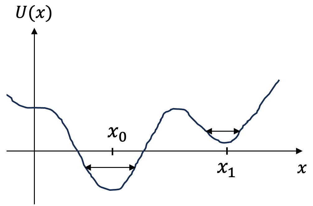
In general, consider a potential energy \(U(x)\) that has a minimum at \(x=x_0\text{.}\) By writing the potential energy function in terms of a Taylor series about \(x=x_0\) we obtain the following.
\begin{equation*}
U(x)= U(x_0) + \left(\frac{dU}{dx}\right)_{x=x_0}\left(x-x_0\right) + \frac{1}{2!}\left(\frac{d^2U}{dx^2}\right)_{x=x_0}\left(x-x_0\right)^2 + \cdots
\end{equation*}
Since the potential energy has a minimum at \(x=x_0\text{,}\) the first derivative is zero there, and the leading non-constant term is the quadratic term in \(x-x_0\text{,}\) the displacement from the equilibrium.
\begin{equation*}
U(x)= U(x_0) + \frac{1}{2!}\left(\frac{d^2U}{dx^2}\right)_{x=x_0}\left(x-x_0\right)^2 + \cdots
\end{equation*}
The value of the second derivative of the potential energy function for \(x=x_0\) is a constant. Let us denote this constant by \(k\) in anticipation of its analogy with the spring constant of a spring.
\begin{equation*}
k \equiv \left(\frac{d^2U}{dx^2}\right)_{x=x_0}.
\end{equation*}
Choosing the potential energy to be zero at the equilibrium, and placing the origin at the equilibrium point, we find that near a potential energy minimum, the leading behavior of the potential energy function is quadratic.
\begin{equation*}
U(x)= \frac{1}{2!}kx^2+\cdots
\end{equation*}
Therefore, even though an oscillating system may not be a block attached to a spring, the behavior is “identical” to the problem of a block attached to a spring and we can speak of a “spring constant” whenever a system is oscillating such that near the bottom of the potential energy the potential energy can be approximated by a quadratic function of the corresponding displacement. The only exceptions are those potential energy functions, such as \(U(x) = b x^4\text{,}\) which cannot be approximated by a quadratic function near the minima.
A quadratic potential energy function gives a linear restoring force of the Hooke’s law and leads to the Simple Harmonic Motion.
\begin{equation*}
F_x= -\frac{dU}{dx}= -k x + (\textrm{ higher powers in }x).
\end{equation*}
We have seen above that the plane pendulum is not a Simple Harmonic Oscillator unless the angle of oscillation is small. We can see this emerging Simple Harmonic property from the perspective of a quadratic potential energy function. The potential energy of a pendulum when it is displaced at angle \(\theta\) is
\begin{equation*}
U = m\, g\, l\, (1- \cos \theta).
\end{equation*}
Now, expanding \(\cos (\theta)\) for small \(\theta\) we find
\begin{equation*}
\cos(\theta) = 1-\frac{1}{2!}\theta^2 + \frac{1}{4!}\theta^4 + ....
\end{equation*}
If we keep only the leading term, viz., \(1\text{,}\) we will lose all physics information associated with \(\theta\text{.}\) Therefore, we will keep two terms in this expansion. This gives the following expression for the potential energy near \(\theta=0\text{:}\)
\begin{equation*}
U = \frac{m g l}{2}\theta^2,
\end{equation*}
which is quadratic in the dynamical variable \(\theta\text{.}\) Hence, for small angles we expect a Simple Harmonic Motion for the pendulum as discussed previously.