Optical instruments such as camera, microscope, and telescope use lenses and mirrors to view and record images of physical objects. They also rely on gathering enough light energy for clear view and the speed with which instrument can be operated. They are often characterized by a few parameters, such as aperture, f-stops, magnifying power, focal length, numerical aperture, etc. Let’s briefly define them here so that we can use them in our discussion of instruments in this chapter.
We have encountered focal length, denoted by \(f\text{,}\) for curved mirrors and lenses. For converging systems, whether a concave mirror or a convex lens, focal length is the distance from vertex to the focal plane where parallel rays from distant objects converge. For diverging systems, i.e., a convex mirror or a concave lens, focal length the distance from vertex to the focal plane where parallel rays from distant objects appear to diverge from.
In the case of curved mirrors, focal length is equal to half the radius of curvature.
\begin{equation*}
f = \frac{R}{2},
\end{equation*}
if light ray “sees” a convex surface and negative if it “sees” a concave surface. In the case of thin lenses, focal length of a lens is air is given by the Lens-maker’s formula.
where \(n_l\) is the refractive index of the lens material and \(R_1\) and \(R_2\) are radii of curvatures which are positve if light ray “sees” a convex surface and negative if it “sees” a concave surface.
With appropriate sign conventions for object distance \(p\text{,}\) image distance \(q\text{,}\) and focal length \(f\) for both mirrors and lenses for arbitrarily placed object, not just objects that are far away, are related by the same equation.
The magnification, also known as transverse magnification, denoted by \(m\) or \(m_T\text{,}\) is given by the ratio of the height of the image \(h_i\) to the height of the object \(h_o\) with appropriate signs, e.g., given by a coordinate axis values \(y_i\) and \(y_o\) with the odd-axis point for height being along the \(y\)-axis. By geometry and sign convenstions, it can also be shown to be equal to ratio of the image distance and object distance.
\begin{equation*}
m = \frac{h_i}{h_o} = - \frac{q}{p}.
\end{equation*}
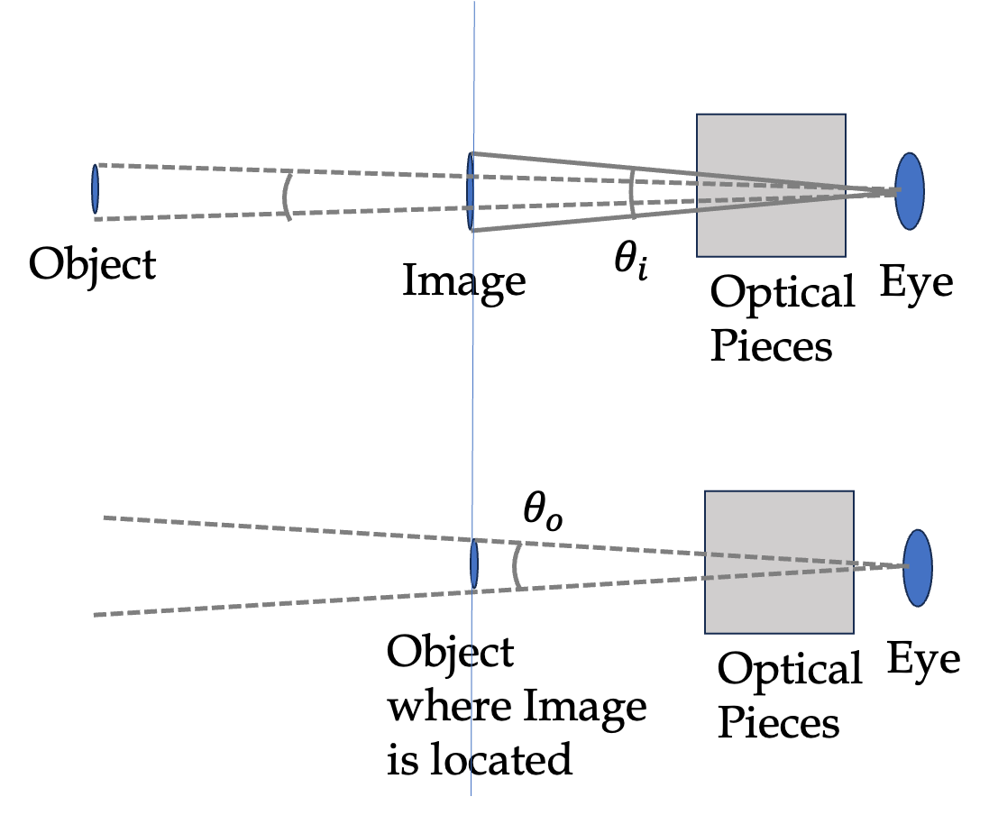
When eye is involved in viewing a virtual image, an angular magnification is more relevant. Angular magnification forcus on the angles subtended at the eye by the object and the image as illustrated in Figure 45.1.
Angular magnification is the ratio of the angle \(\theta_i\) subtended by the image at the eye to the angle \(\theta_o\) submitted, not by the original object but by the object placed at the same distance as the image. We denote angular magnification by \(M\text{.}\)
\begin{equation*}
M = \frac{\theta_i}{\theta_o}.
\end{equation*}
Figure45.1.
Eye can see an object clearly at a distance about \(25\text{ cm}\text{.}\) This is called near point of the eye. I will desnote this distance by \(n_p\text{.}\) The angular magnification of a converging lens of focal length \(f\) will be shown to be
Magnification of a multi-lens system comes from multiplying magnifying power of each one. For instance, in a microscope, the magnifying power of the microscope is a product of the magnification of the objective and the angular magnification of the eyepiece.
Light can enter an instrument through some opening called aperture. The area \(A\) of the aperture is an important characteristic of an instrument as it gives us a way to quantify amount of light energy that can enter the system. Recall that intensity \(I\) of light is energy per unit time per unit area. Therefore, a product of intensity and area of the aperture is the energy entering the apparatus per unit time.
\begin{equation*}
\text{Energy per unit time entering apparatus} = I\,A.
\end{equation*}
Often, the opening through which light enter an instrument is circular. In that case, in place of aperture area, we give aperture diameter, \(D\text{,}\) which is the diameter of the aperture stop. Of course, you can get area from it immediately.
\begin{equation*}
A = \frac{\pi}{4} D^2.
\end{equation*}
In a reflecting telescopes, usually a concave mirror collects light. So, if you have an \(8\text{-in}\) telescope, it means that you have \(D=8\text{ inches}\text{.}\) Due to the square of diameter in the formula for area, a \(16\text{-in}\) telescope will gather \(4\) times as much light, and therefore, you will be able to see much fainter object.
In many instruments, light is restricted to be near the axis of the instrument by using a light blocker with a hole. This object is called aperture stop. See Figure 45.2. Stops are used to reduced image blurring due to aberrations.
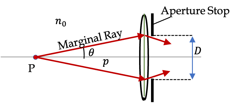
When you place an object on the axis in front of the entrance of an instrument, the ray with the largest angle that can enter the instrument is called Marginal Ray as illustrated in Figure 45.2. The angle of the marginal ray is an important characteristic of an instument. A quantity, numerical aperture, is defined based on this angle and the refractive index of the ambient medium.
Consider a lens with object at point P on the axis. Let \(n_0\) be the refractive index of the ambient around P as shown in Figure 45.2. Let there be an aperture stop of diameter \(D\) behind the lens. Then, we define numerical aperture as
Figure45.2.Aperture, aperture stop and marginal rays.
If you don’t have any aperture stop, then you can think of light being collectd from the entre lens; that will mean the value of \(D\) will equal the diameter of the lens itself in that case. Using the geometry in Figure 45.2, you can express \(\text{NA}\) also as
If we further assume that angle \(\theta\) is small so that \(\sin\theta \approx \theta\) ; this will coincide with the case of \(D \ll p\text{.}\) Then, we will further simplification:
In Eq. (45.2), if you place the object at the focal point of the lens, i.e., when \(p=f\text{,}\) you will get a characteristic numerical aperture, which we will denote by attaching a subscript \(f\) to \(\text{NA}\text{.}\)
Thus, we see that ability of light to enter the instrument can be characterized by the ratio of diameter of the aperture and the focal length. We note that larger value of \(D/f\) will mean more light enters the apparatus. Larger \(D/f\) would mean we can collect same amount of light in less time. The inverse of this, i.e., \(f/D\text{,}\) is called the F/Number or F-Stop. F/Number is more commonly written as F/#.
\begin{equation}
\text{F/\# or F-stop} = \frac{f}{D}.\tag{45.3}
\end{equation}
In terms of numerical aperture at focal length, this becomes
\begin{equation*}
\text{F/\# or F-stop} = \frac{n_0}{\text{NA}_f}.
\end{equation*}
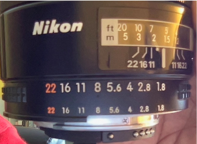
The term F-Stop is more common name for this parameter in cameras, where it is set by selecting the diameter of an aperture stop since focal length is fixed. F-Stop (F/#) are opposite of light collection ratio \(D/f\text{.}\) Smaller F/# or F-Stop corresponds to collection of more light per sec, which will mean smaller F/# or F-Stop is a faster system than one with higher higher F/# or F-Stop.
Figure45.3.
Subsection45.1.4Power of Stacked Lenses
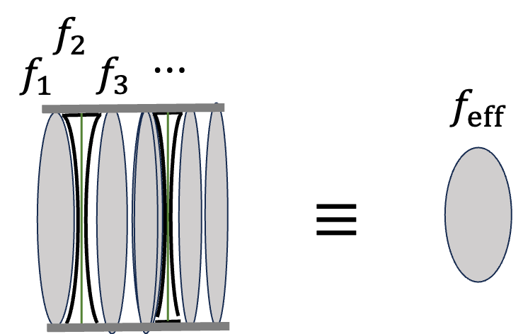
In many instruments, lenses are stacked together as shown in Figure 45.4. For a detail ray tracing, you need to work rays through all the lenses as we have done for two-lens systems we have studied before. But, if the lenses are stacked together, we can simplify our work and replace all the lenses with one lens if we do not need to worry about either the thickness of the lenses or separation between them.
Figure45.4.
In this approximation, you can show that the effective focal length is related to the focal lengths of the individual lenses as follows.
Remark45.5.Derivation of the Power Addition Formula for Two Lenses.
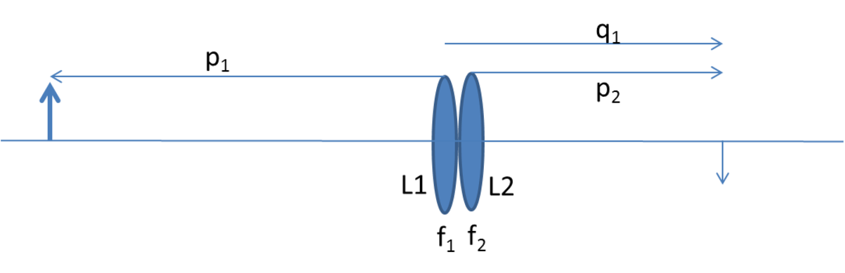
Consider a two-lens situation depicted in Figure 45.6.
Figure45.6.
The figure shows the physical situation. We will work out the image distance due to the first lens L\(_1\) and then use that intermediate image as a virtual object for the second lens L\(_2\text{.}\)
2.Angular Magnification for Convex Lens if Eye Very Close.
What will be the formula for the angular magnification of a convex lens if the eye is very close to the lens and the near point is located a distance \(D\) from the eye?
Solution.
We just have to replace \(25\,\text{cm}\) by \(D\text{.}\)
\begin{equation*}
M = 1 + \dfrac{D}{f}.
\end{equation*}