   
Logo image

Physics Bootcamp

Section 40.5 Power Delivered by the Source

The practical importance of the resonance phenomenon is seen dramatically in the choice of the frequency of the driving power source in delivering power to the rest of the circuit. The energy at any instant is stored in the capacitor and the inductor, but only the resistor in the circuit dissipates energy. Therefore, the average energy used by the circuit during an interval will be equal to the product of the instantaneous power into the resistor and the interval of time. Thus, the energy deposited in the resistor in an interval of time between \(t\) to \(t+dt\) will be given by
\begin{equation*} P(t) dt = I(t) V_R(t), \end{equation*}
where \(I(t)\) is the current through the resistor and \(V_R\) is the voltage drop across the resistor. From Ohm’s law we can replace \(V_R\) by \(I R\) and obtain
\begin{equation*} P(t) dt = I_0^2 R\cos^2(\omega t+\delta), \end{equation*}
where \(\delta\) is the phase of the current relative to the phase of the driving EMF. The energy deposited in the resistor per cycle is obtained by integrating this expression over a period, \(T = 2\pi/\omega\text{.}\)
\begin{equation*} \textrm{Energy(one cyle)}=\int_0^{T}P(t) dt = \frac{1}{2}I_0^2 RT. \end{equation*}
Therefore, the average rate at which the energy is dissipated in the resistor will be \(\frac{1}{2}I_0R^2\text{.}\) This is the average power dissipated.
\begin{equation} P_{\textrm{ave}} = \frac{\textrm{Energy(one cyle)}}{T} = \frac{1}{2}I_0^2R.\tag{40.45} \end{equation}
Since the peak current \(I_0\) is a function of the driving frequency \(\omega\text{,}\) the average power delivered would also be a function of the frequency \(\omega\) of the EMF source. Thus, the average power is maximum at the same frequency at which the peak current is maximum. We saw above that the peak current was maximum when the source EMF was oscillating at the same frequency as the natural frequency of the circuit. 
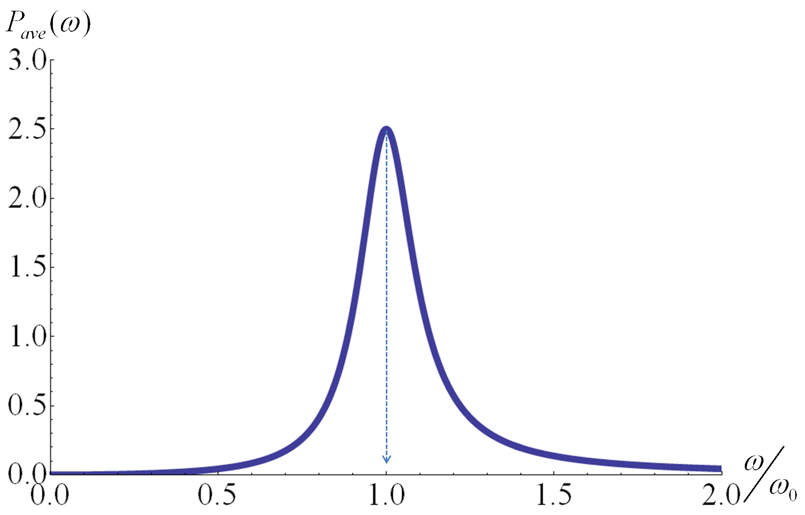
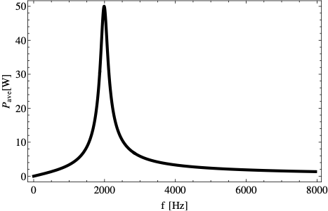
Figure 40.45 shows the resonance curve of average power.
Figure 40.45. The resonance curve of the average power dissipated in the resistor for \(R\) = 0.2 \(\Omega\text{,}\) \(L\)= 1 H, \(C\) = 1 F, and the peak voltage of the driving EMF set to \(V_0 = 1\) V. The peak power is delivered when the driving frequency \(\omega\) is equal to the natural frequency \(\omega_0\) of the circuit.
The curve shows that the maximum power is delivered to the circuit when the circuit is driven at the natural frequency. Denoting the resonance frequency of power as \(\omega_R\) we have
\begin{equation*} \omega_R = \omega_0 = \frac{1}{\sqrt{LC}}\ \ \ \textrm{(Resonance of Power.)} \end{equation*}
This formula for the average power in the resistor differs from the power for the constant current circuit we had found in an earlier chapter. There, we had found that the power dissipated in a resistor is \(I^2R\text{,}\) but here we find that the average power is \(\frac{1}{2}I_0^2R\) where \(I_0\) is the amplitude of the oscillating current, which changes between \(-I_0\) and \(+I_0\) sinusoidally in time. It is possible to define an averaged current, called the {\bf root-mean squared current}, or the {\bf RMS-current}, \index{RMS current} we can rewrite the average power \(P_{\textrm{ave}}\) as a formula that is similar to a DC circuit.
\begin{equation*} I_{\textrm{rms}} = \frac{I_0}{\sqrt{2}} \end{equation*}
This will give the average power dissipated as
\begin{equation*} P_{\textrm{ave}} = R\: I_{\textrm{rms}}^2. \end{equation*}

Example 40.46.

For each circuit in Figure 40.27, find the average power delivered to the circuit if the peak voltage of the source of frequency 600 Hz is 10 V.
Solution.
Average power is related to the peak current and resistance only: \(P_{\textrm{ave}} = \frac{1}{2}RI_0^2\text{,}\) where \(I_0\) is the peak current. The peak current for each circuit has been worked out in the last exercise. Now, using this formula we obtain the following values for the average power: (a) \(0.8\, \text{W}\text{,}\) (b) \(2.7\, \text{W}\text{,}\) (c) \(0.011\, \text{W}\text{,}\) and (d) \(14\, \text{W}\text{.}\)

Exercises Exercises

1. Average Powerer Delivered to a Circuit at Different Frequencies.

For circuit (a) in Figure 40.27, find the average power delivered to the circuit by a \(10\text{-V}\) source at following frequencies, plot the average power delivered versus frequency, and compare the peak frequency with the resonance frequency of the circuit: (a) \(100\, \text{Hz}\text{,}\) (b) \(300\, \text{Hz}\text{,}\) (c) \(500\, \text{Hz}\text{,}\) (d) \(700\, \text{Hz}\text{,}\) (e) \(1000\, \text{Hz}\text{,}\) (f) \(2500\, \text{Hz}\text{,}\) (g) \(4500\, \text{Hz}\text{,}\) (h) \(6000\, \text{Hz}\text{,}\) (i) \(8000\, \text{Hz}\text{,}\) and (j) \(10000\, \text{Hz}\text{.}\)
Solution.
Since impedance depends on the frequency of the driving EMF, the current will also depend on the frequency. Hence, the average power delivered will also be a function of frequency of the driving EMF. We can better organize the answer in a table.
Table 40.47.
\(f\, (\text{Hz})\) \(Z\, (\Omega)\) \(I_0\,(\text{mA})\) \(P_\text{ave}\,(\text{mW})\)
(a) \(100\) \(394\) \(25\) \(13\)
(b) \(300\) \(121\) \(83\) \(140\)
(c) \(500\) \(63\) \(160\) \(510\)
(d) \(700\) \(42\) \(240\) \(1100\)
(e) \(1000\) \(46.2\) \(220\) \(940\)
(f) \(2500\) \(147\) \(68\) \(93\)
(g) \(4500\) \(277\) \(36\) \(26\)
(h) \(6000\) \(372\) \(27\) \(14\)
(i) \(8000\) \(499\) \(20\) \(8\)
(j) \(10000\) \(626\) \(16\) \(5.1\)
Plot the data to obtain the power versus frequency plot. You would find a peak power. Read the resonance frequency from your plot and compare to the calculated value.

2. Power Dissipating in Resistor of a Driven RLC Circuit.

For circuit (c) in Figure 40.27, plot the average power dissipated in the resistor versus frequency of a 10-V source. (b) At what value of the frequency is the maximum power dissipated?
Solution 1. a
The formula for average power dissipated can be expressed as a function of frequency \(f\) as follows.
\begin{equation*} P_{\textrm{ave}} = \dfrac{\frac{1}{2}RV_0^2}{R^2 + (2\pi f L - 1/2\pi f C)^2}.\quad (1) \end{equation*}
We now put the numerical values given in circuit (c) in Figure 40.27 and plot \(P_{\textrm{ave}}\) versus \(f\text{.}\)
Figure 40.48.
Solution 2. b
The power is greatest when the denominator in (1) is the smallest. This takes place at the frequency
\begin{equation*} f_R = \dfrac{1}{2\pi\sqrt{LC}} = 1989\:\textrm{Hz}. \end{equation*}