Vectors as Arrows

Section 3.1 Vectors as Arrows

A vector can be represented by an arrow of appropriate size and in appropriate direction. For instance, a position vector will be an arrow from the origin to the location of the object in space. A velocity vector will be an arrow in velocity space. A force vector, similarly, will be an arrow in another abstract space we will call force space.

As usual, we will place an arrow over a symbol to represent the vector while we will use the symbol itself for the magnitude of the vector. For instance, we can represent a displacement vector by \(\vec D\) and its magnitude by \(D\) and sometimes by surrounding the vector symbol with an absolute sign, e.g., \(|\vec D|\text{.}\) Similarly, \(\vec v\) for velocity and \(v\) or \(|\vec v|\) for the magnitude of the velocity, i.e, speed.

\begin{equation} \text{Notation: Vector }\vec A\text{ has magintude denoted by } A\text{ or }|\vec A|.\tag{3.1} \end{equation}

The absolute symbol around the vector name is suposed to emphasize that the magnitude is alwys a positive number.

Subsection 3.1.1 Drawing Vector Arrows

Supposeyou drive from point A to point B such that direct distance between A and B is \(2.0\text{ km}\text{.}\)

We will take a displacement vector in the ordinary space as our running example to illustrate various concepts.

Then, we can draw an arrow of \(2\text{ cm}\) in the direction from A to B to represent the actual displacement using a scale \(1\text{ cm} \equiv 1\text{ km}\) as shown in Figure 3.1. The figure also shows a second displacement vector from B-to-C whose length corresponds to \(3.0\text{ km}\text{.}\)

Figure 3.1. To draw an arrow for a vector, you need to decide on SCALE first. Then, you know the size of the arrow to draw. Now, you would draw all vectors of that type using the same scale in the same diagram. We have two displacement vectors here A-to-B and B-to-C.

An important feature of an arrow representing a vector is that ALL VECTORS THAT HAVE THE SAME SIZE AND SAME ORIENTATION are equal to each other. So, the displacement from A to B will equal from X to Y in the diagram even though they have been drawn at different places beacuase they have the same size and same direction in space. But, A-to-B vector is not equal to P-to-Q vector even though they have the same size. Can you tell why?

Subsection 3.1.2 Multiplication of a Vector by a Scalar

A scalar is any real number, positive, negative, or zero. The effect of multiplying a vector by a scalar is very different for positive and negative scalars. Multiplication of a vector \(\vec A\) by a scalar \(s\) gives a new vector \(\vec B = s\vec A\text{.}\)

If \(s\) is a positive scalar, then \(\vec B\) has the same direction as \(\vec A\) but its magnitude is \(s\) times the magnitude of \(\vec A\text{.}\) That is, \(|\vec B| = s|\vec A|\text{.}\) If \(s \gt 1\) then \(|\vec B|\) is \(s\) times greater and if \(s \lt 1\) then \(|\vec B|\) is \(s\) times smaller.

Note that dividing by the scalar \(s\) is equivalent to multiplying by \(1/s\text{,}\) so the division is not a different operation than multiplication. We can obtain a vector of any length in the same direction as the original vector by multiplying it by an appropriate positive real number.

Multiplication of a vector \(\vec A\) by a negative number \((-s)\) [minus \(s\)] gives a new vector, denoted by \(\vec C\) here, that is \(s\) times the original vector but also its direction is opposite to the direction of \(\vec A\) (Figure 3.3). For instance, when velocity vector of \(10\) m/s pointed North is multiplied by \(-2\text{,}\) you get another velocity vector that has a magnitude \(20\) m/s and pointed South.

Subsection 3.1.3 Unit Vector

Evidently dividing a vector \(\vec A\) by its magnitude \(|\vec A|\) one should obtain a vector whose length is \(1\) with no units and the same direction as the direction of vector \(\vec A\text{.}\) This vector is called unit vector in the direction of \(\vec A\text{.}\) We will denote unit vectors obtained this way by placing a karat over the symbol of the original vector, \(\hat A\text{.}\) Thus, unit vector \(\hat A\) is

\begin{equation} \boxed{\hat A = \frac{\vec A}{|\vec A|}.}\tag{3.2} \end{equation}

Unit vectors are very useful for constructing vectors of arbitrary lengths. For instance, if we want a displacement vector of length \(5\) cm in the direction of some unit vector \(\hat u\text{,}\) then all we need to do is to multiply \(\hat u\) by \(5\ cm\text{,}\) giving the desired vector \((5\ \text{cm})\hat u\text{.}\) Now, a force vector of length \(10\) N in the same direction as \(\hat u\) will be \((10\ \text{N})\hat u\text{.}\) You can see that unit vectors have universal applicability regardless of how you construct them. They are holders of the information about directions in space. As you might have guessed it, there are infinite number of unit vectors, one for each direction in space.

Subsection 3.1.4 Adding Vector Arrows

In Figure 3.1, we have two displacements A-to-B, denoted by the name \(\vec D_1\text{,}\) and B-to-C, denoted by \(\vec D_2\text{.}\) What will be the net displacement? That is, what we want to know is: if you go from A-to-B and then go from B-to-C, what is your net displacement?

From the definition of displacement, the net displacement depends only on the initial and the final points. An arrow from the initial point to the final point will be the net displacement arrow. Here, the net displacement will be the direct arrow from A-to-C. Let’s denote this vector by \(\vec D_3\text{.}\) Thus, we have added vectors \(\vec D_1\) and \(\vec D_2\) and the result is \(\vec D_3\) as shown in Figure 3.4.

How do we figure out the magnitude and direction of the sum vector \(\vec D_3\text{?}\) First, we read off the length of the arrow from A to C and use the scale. In my original drawing I had used 1 cm to represent 1 km. The size of the arrow on the diagram turned to be 2.6 cm, which would correspond to 2.6 km. Clearly, the sizes don’t add since \(2.6 \ne (2.0 + 3.0)\text{.}\)

For telling the direction of \(\vec D_3\text{,}\) we can use the angle with respect to, say, vector \(\vec D_1\text{.}\) I used a protractor to get the angle.

The procedure of adding vectors illustrated in Figure 3.4 goes by the name parallelogram law of addition. Why is it called parallelogram law? The name comes from the way the vectors to be summed form sides of a parallelogram and one of the diagonals gives the sum as illustrated in Figure 3.5. The other diagonal gives the difference.

In Figure 3.4, (a) Tip-to-tail method: place one vector after another keeping the orientation in space unchanged while you move the second vector. The diagonal from the tail of the first vector to the tip of the second vector is sum. The difference is the other diagonal. (b) Tail-to-Tail method: Place tails of both vectors at the same point. Again keep the original directions in space unchanged. The diaginal from the common tail is the sum.

Figure 3.5. Parallelogram law of addition of vectors.

The parallelogram law of addition can be extended to the addition of more than two vectors by simply placing each additional vector starting from the tip of the last vector added as illustrated in Figure 3.6. First we add two of the vectors as shown in (b), getting \(\vec V_{12}\) from \(\vec V_1\) and \(\vec V_2\text{.}\) And then, we add the third vector to the sum of the first two as shown in (c) to get \(\vec V_{123}\text{.}\)

Figure 3.6. Addition of more than two vectors.

Example 3.7. Zero Vector and Negative of a Vector.

What will happen if you add two vectors that have exactly the same magnitude but their directions are oposite to each other? As if you walked from A to B and then you walked back to A. What will be the net displacement. Clearly, you will get zero displacement. Thus adding two equal size but oposite direction vectors gives you a “vector” of zero size. The direction of a zero size vector is not defined.

As an equation, let \(\vec A\) be the first vector and \(\vec B\) be the vector equal in size to \(\vec A\) but in oposite direction. Then, we have the following result when we add them.

\begin{equation*} \vec A + \vec B = \vec 0, \end{equation*}

where I have placed an arrow over zero just to remind us that we are not doing ordinary addition but rather a vector addition. Now, we can move \(\vec A\) on the other side of the equation to see that this opposite to \(\vec A\) is nothing but negative of \(\vec A\text{.}\)

\begin{equation*} \vec B = \vec 0 - \vec A = -\vec A. \end{equation*}

That is negative of a vector gives another vector that has the same magnitude but has exactly the oposit edirection.

Example 3.8. Vectors as Sum of Vectors along Cartesian Axes.

Now, that we have learned how to add two vectors, let us demonstrate that in \(xy\)-plane, any vector can be written as a sum of two vectors, one along the \(x\)-axis and the other along the \(y\)-axis. You can easily extend this example to the three-dimensional soace.

In Figure 3.9, vector \(\vec D\) is sum of vector \(\vec D_x\) and \(\vec D_y\text{.}\) You can see this easily from the parallelogram (here rectangle) PQRS, where the original vector \(\vec D\) is along the diagonal and \(\vec D_x\) and \(\vec D_y\) along the axes.

\begin{equation*} \vec D = \vec D_x + \vec D_y, \end{equation*}

where magnitudes of \(\vec D_x\) and \(\vec D_y\) are \(D_x = D \cos\theta\) and \(D_y = D\sin\theta\text{.}\)

Example 3.10. Three Forces Acting at Three Points on a Ring.

Three forces act at three points on a ring such that their directions are in one plane and their vector arrows all fall in that plane. We will use one of the forces to indicate the directions of the other two. The forces are: \(3\) N force in some direction in the plane, \(6\) N force in a direction that is \(60^{\circ}\) counterclockwise from the direction of the \(3\)-N force and \(4.5\) N force that is acting \(90^{\circ}\) clockwise from the direction of the \(3\)-N force. Graphically add the given force vectors by drawing them in a tip-to-tail way, and find the magnitude and direction of the sum force, also called the net force.

Solution.

The graph and the steps to construct the graph are displayed in Figure 3.11

Subsection 3.1.5 Subtraction of Vectors

Subtracting a vector \(\vec B\) from another vector \(\vec A\) can be turned into adding the negative of vector \(\vec B\) to \(\vec A\text{.}\)

\begin{equation*} \vec A-\vec B = \vec A + \left(-\vec B\right). \end{equation*}

Geometrical procedure of \((\vec A-\vec B)\) this subtraction is illustrated in Figure 3.12.

First draw vectors \(\vec A\text{,}\) \(\vec B\text{,}\) and \((-\vec B)\text{.}\) Then, we can proceed in two ways to find the vector that is equal to \((\vec A-\vec B)\text{:}\)

(a) At the tip of vector \(\vec A\) draw the vector \((-\vec B)\text{,}\) which is obtained from vector \(\vec B\) by reversing the direction of the later. From the tail of \(\vec A\) to the tip of \((-\vec B)\) is the vector \((\vec A-\vec B)\text{.}\)

(b) You would obtain the same result for \((\vec A-\vec B)\) by drawing \(\vec B\) such that its tip meets the tip of \(\vec A\text{.}\) Then \((\vec A-\vec B)\) is from the tail of \(\vec A\) to the tail of \(\vec B\text{.}\)

Subsection 3.1.6 Vector Equations and Polygons

Recall that when you walk around a polygon and end up at the starting place, then your direct distance from the starting place to ending place is zero. This means that the net displacement must be a zero vector, also called the null vector. Thus, if you add vectors by placing the tail of one vector at the tip of another vector and the result is a closed polygon, the net sum of all vectors will be zero vector as illustrated in Figure 3.13.

Figure 3.13. Polygon of vectors arranged tip-to-tail add up to zero or null vector.

Therefore, for any polygon of vectors we can write a vector equation. In Figure 3.13(a), the three vectors give rise to the vector equation

\begin{equation*} \vec V_1 + \vec V_2 +\vec V_3 = 0, \end{equation*}

which is the same as

\begin{equation*} \vec V_1 + \vec V_2 = (-\vec V_3), \end{equation*}

which shows that the sum of the two vectors \(\vec V_1\) and \(\vec V_2\) is equal to the vector \((-\vec V_3)\text{,}\) i.e. another vector that has the same magnitude as vector \(\vec V_3\) but has an opposite direction to that of vector \(\vec V_3\text{.}\) Similarly, Figure 3.13(b) corresponds to the vector equation

\begin{equation*} \vec V_1 + \vec V_2 +\vec V_3 +\vec V_4 = 0. \end{equation*}

You will find many vector equations in this textbook. For example, the second law of motion is a vector equation \(\vec F = m\vec a\text{,}\) which says that the force vector obtained by vector addition of all the forces on the object of mass \(m\) is equal to the vector obtained by multiplying the acceleration vector with the mass.

Subsection 3.1.7 Projection of one Vector Over Another

Often we need to know “how much” of a vector \(\vec B\) acts in the direction of another vector \(\vec A\text{.}\) This quantity is called the projection of \(\vec B\) over \(\vec A\text{.}\) A related quantity of interest is “how much” of a vector \(\vec B\) acts in the direction of perpendicular of another vector \(\vec A\text{.}\)

Figure 3.14 illustrates how to find projections by drawing two vectors from a common tail point. When you draw a normal to the line of \(\vec A\) from the tip of \(\vec B\text{,}\) you strike that line either on the side of \(\vec A\) as in Figure 3.14(a) or in the opposite to \(\vec A\) as in Figure 3.14(b). The distance from the common tail to the point of normal on the line of \(\vec A\) is the projection of \(\vec B\) on \(\vec A\text{.}\) In the case of (a), the projection will be positive and in the case of (b) it will be negative.

In Figure 3.14, I have denoted projection of \(\vec B\) on \(\vec A\) by the symbol \(B_{\parallel A}\) to indicate that this is the part of \(\vec B\) that is acting in the direction of \(\vec A\text{.}\)

If you draw projection of \(\vec B\) on a direction perpendicular to \(\vec A\text{,}\) you would get another projection value, which I have denoted by \(B_{\perp A}\text{.}\) Actually, these symbols for projections are not universally followed. As a matter of fact, many people use confusing symbol \(B_\perp\) to denote the projection of \(\vec B\) on \(\vec A\text{.}\) We also might do that sometimes. It should be clear from the context.

Subsection 3.1.8 Multiplication of a Vector with Another Vector

You have already learned what happens when you multiply a vector by a real number (also called a scalar). How do you multiply a vector by another vector? A vector has a numerical part in the magnitude and a non-numerical part in the direction. For instance, a velocity vector can be \(3\) m/s East and another velocity can be \(4\) m/s Up. Granted you can think of a way to multiply \(3\) and \(4 \text{,}\) but how would you multiply East and Up?

It turns out that two types of multiplication are found in physics. (1) In one type of multiplication, called the scalar product, the product of two vectors is actually a scalar number that depends upon the magnitudes of the two and the angle between them. We call this type of multiplication a scalar product. Examples of this type of multiplication are work and energy. (2) In the other type of multiplication between two vectors, called the vector product, the product is another vector. Examples of this vector products are torque and angular momentum.

Subsubsection 3.1.8.1 Scalar Or Dot Product

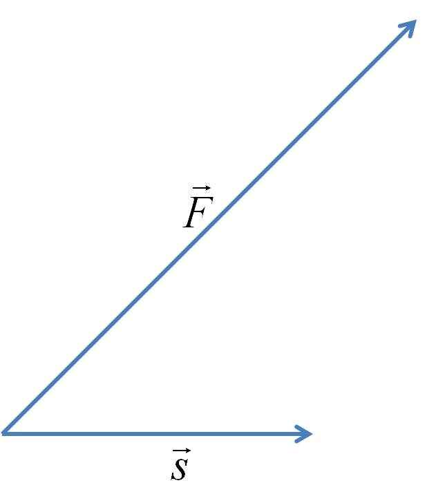
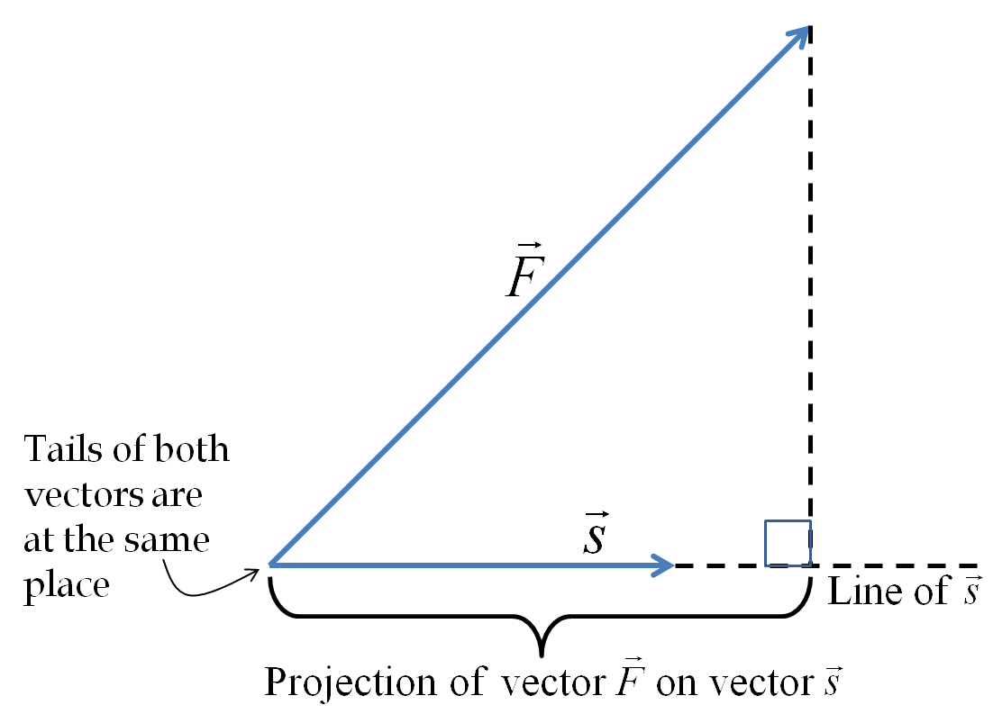
The scalar product of two vectors \(\vec A\) and \(\vec B\) is defined by the product of the magnitude of one these vectors and the projection of the other vector along this vector. It’s denoted by the composite symbol “\(\vec A \cdot \vec B\)”.

\begin{equation} \vec{A} \cdot \vec{B} = |\vec{A}| \times \text{Projection of }\vec{B}\text{ on }\vec{A} \equiv A B_{\parallel A},\tag{3.3} \end{equation}

or, equivalently.

\begin{equation} \vec A \cdot \vec B = |\vec B| \times \text{Projection of }\vec A\text{ on }\vec B \equiv B A_{\parallel B}.\tag{3.4} \end{equation}

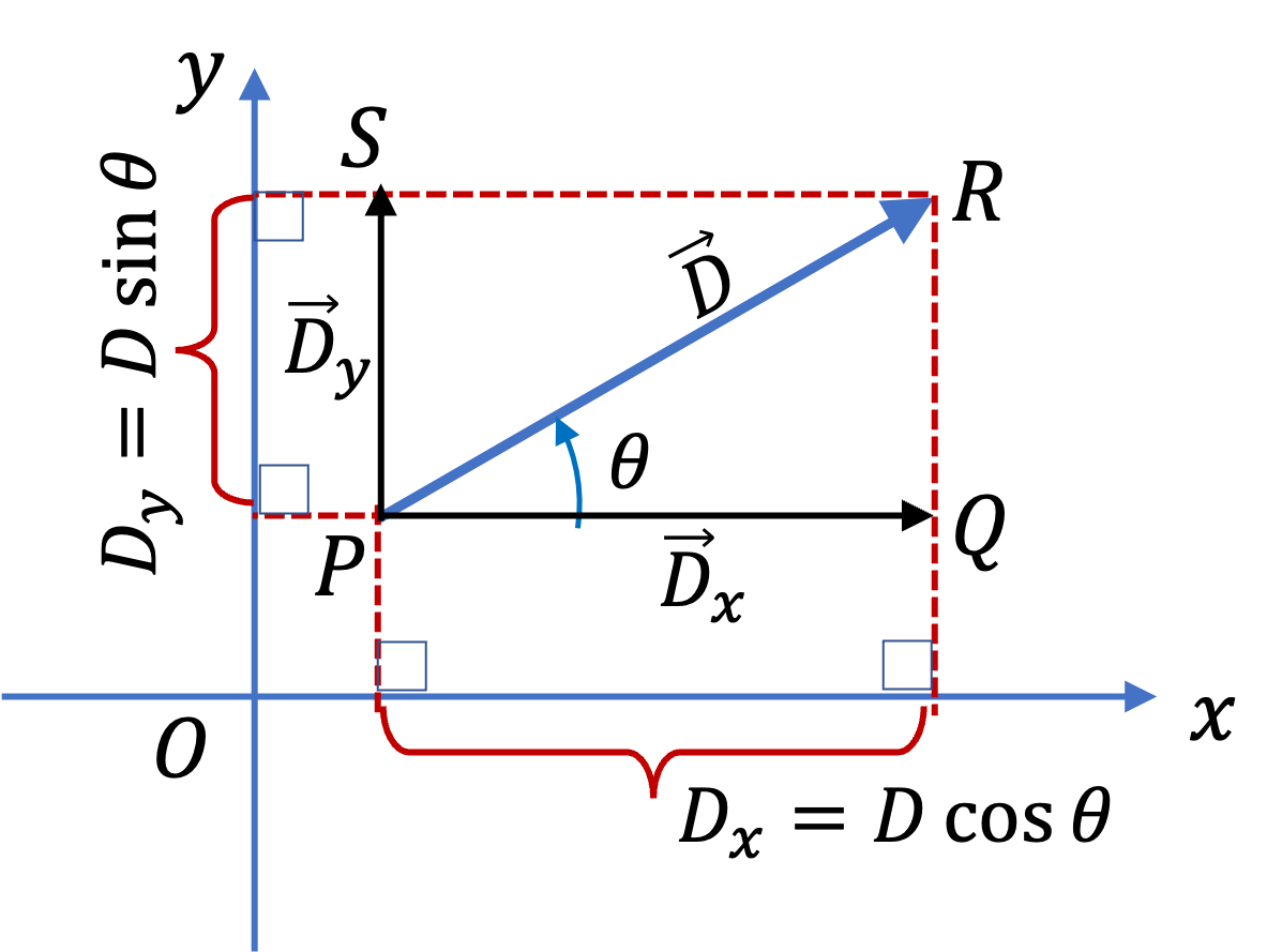
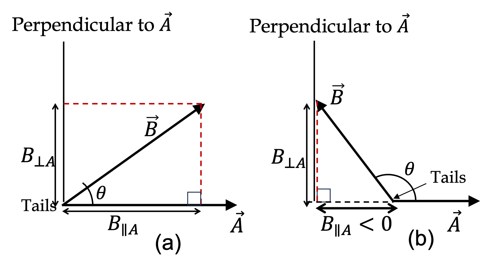
Refering to Figure 3.14, we see that we can use trigonometry of right-angled triangle to write the projection of \(\vec B\) on \(\vec A\) in terms of the angle \(\theta\text{.}\)

\begin{equation} B_{\parallel A} = B\,\cos\theta.\tag{3.5} \end{equation}

This formula covers both the positive and negative projections since \(\cos\theta\) is negative for \(90^\circ \lt \theta \lt 270^\circ\text{.}\) Therefore, we can also write the following for the scalar product.

\begin{equation} \vec A \cdot \vec B = A B\cos\theta.\tag{3.6} \end{equation}

Note that if the dot product between two vectors is zero, then, either one or both of the vectors has a zero length, or the angle between them in ninety degrees since \(\cos 90^{\circ} = 0\text{.}\)

\begin{equation*} \boxed{\text{If}\ \vec A\cdot \vec B = 0, \text{ then, either }|\vec A| = 0, \text{ or } |\vec B| = 0, \text{ or }\theta = 90^{\circ}.} \end{equation*}

Another useful property of the scalar product occurs when you take the scalar product of a vector with itself. Since \(\cos\theta = 1\) here, or equivalently, the projection of a vector on itself will be the entire magnitude of the vector, the scalar product is equal to the square of the magnitude of the vector.

\begin{equation*} \vec A\cdot\vec A = |\vec A|^2. \end{equation*}

Based on the definition of the scalar product given above, you can prove the following algebraic properties of the scalar product.

Linearity: \(\vec A \cdot(s\vec B) = s \vec A\cdot \vec B\text{,}\) where \(s\) is scalar.
Distributive: \(\vec A\cdot(\vec B+ \vec C) = \vec A\cdot\vec B + \vec A\cdot\vec C\text{.}\)
Commutative: \(\vec A \cdot\vec B = \vec B \cdot\vec A\text{.}\)

Example 3.15. Projection of Vectors and Scalar Product.

A force \(\vec F\) of magnitude \(10\) N and a displacement \(\vec s\) of magnitude \(10\) cm are shown to their corresponding scales in Figure 3.16. To work graphically on the given vectors, it may be helpful to transfer the figure to another paper using the same scale.

Determine the scales for the two vectors that was used for the given drawings, i.e., state the length of the force arrow that represents \(1\) N of force and the length of the displacement arrow that represents \(1\) cm of displacement. Since the figure shows two different properties we have two different scales, one for each property.
Draw the projection of the force vector on the displacement vector, and determine the value of the projection of the force vector onto the displacement vector in the unit of N.
Draw the projection of the displacement vector on the force vector, and determine the value of the projection of the displacement vector onto the force vector in the unit of cm.
Verify that the product of the projection of \(\vec F\) on \(\vec s\) with the magnitude of \(\vec s\) is equal to the product of the projection of \(\vec s\) on \(\vec F\) with the magnitude of \(\vec F\) within the margin of error of your measurements of the projections.

Solution 1. a

I placed a ruler on the arrow for the force and found the length of the arrow to be 7.5 cm. [Note: the printing of the book on other dimensions will change the length you measure, but the logic given here will not change.] Since this arrow represents a force of magnitude 10 N, the scale for the force in this diagram is 0.75 cm for 1 N.

The reading on the arrow for the displacement gave me a length of 4 cm, which is supposed to represent an actual distance of 10 cm. Therefore, the scale for the distance is 0.4 cm for an actual distance in space of 1 cm.

Solution 2. b

To draw the projection of the vector \(\vec F\) onto the vector \(\vec s\) we need to start with both vectors drawn from the same point as is the case here. Then, we draw a normal line from the tip of the vector \(\vec F\) onto the line of the vector \(\vec s\) that is perpendicular to the the later. Here we need an extension of the line \(\vec s\) forward; some other times you will not have to extend the lines of \(\vec s\) or extend the line backward.

The length from the common tail point to the point on \(\vec s\) where the normal line intersects is equal to the projection of vector \(\vec F\) on vector \(\vec s\) and has the units of the vector \(\vec F\text{.}\) Even though the length projection of the vector \(\vec F\) on the vector \(\vec s\) is along the line of \(\vec s\text{,}\) the projection contains information of the component of the force in the direction of the the vector \(\vec s\) and therefore, this projection has the units of force here. Therefore, the magnitude of the projection will be obtained by using the scale for \(\vec F\) on the projection.

I found the length of the projection is equal to 5.3 cm, which using the scale of 0.75 cm per N gives the projection to be 7.1 N. The projection is positive since the projection normal line intersects the vector \(\vec s\) on the side that is along the the direction of the vector \(\vec s\text{.}\) If the projected line had crossed on the other side of vector \(\vec s\) , then the projection would have been negative.

Solution 3. c

We follow a similar procedure for drawing the projection of the vector \(\vec s\) on the vector \(\vec F\) as we did for drawing the projection of the vector \(\vec F\) on the vector \(vec s\text{.}\) But this time, we use the scale for the distance to convert the length of the projection in the figure to the physical distance of the projection. This gives the projection equal to \(6.5\) cm. In my measurements I got the length of the projection \(2.6\) cm, which using the scale of \(0.4\) cm on drawing equal to \(1\) cm in real space gives the distance \(6.5\) cm in the real space.

Solution 4. d

Let us verify the given statement,

\begin{equation*} \text{Is (Projection of on )} \times |\vec s| = \text{Is (Projection of on )} \times |\vec F|? \end{equation*}

\begin{align*} \amp \text{Left side}\ = 7.1\ \text{N} \times 10\ \text{cm} = 71\ \text{N.cm}\\ \amp \text{Right side}\ = 6.5\ \text{cm} \times 10\ \text{N} = 65\ \text{N.cm} \end{align*}

This says that the left side is not equal to the right side althogh they are supposed to be equal to each other. You can trace the problem in the error in the measurements required in the graphical method. Had I taken the uncertainties into account I would have found that the two values are within the uncertainties of each other.

Subsubsection 3.1.8.2 Vector or Cross Product

The other product of interest to us is the vector product, which is often called the cross product. Unlike the result of the scalar product, the result of a vector product is another vector, whose magnitude depends upon magnitudes of the two vectors and the angle between them, and whose direction depends on the orientations of the two vectors being multiplied. So, to define the vector product, we need rules for the magnitude as well as the direction for the product.

The vector product or the cross product between two vectors \(\vec A\) and \(\vec B\) is another vector, denoted by “\(\vec A\times\vec B\)”, whose magnitude is the area of the area of the parallelogram formed by placing the two vectors on the sides of the parallelogram.

\begin{equation*} \left| \vec A\times \vec B \right| = \text{Area of parallelogram,} \end{equation*}

and the direction of the vector product is given by a rule, called the right-hand rule, illustrated in Figure 3.19.

The magnitude of the vector product is the area of the parallelogram Oacb, which can be written in terms of the magnitudes \(A\) and \(B\) and angle \(\theta\) by recalling the base times height formula. If you take the base to be the side \(A\text{,}\) then the height will be \(B\sin\theta\text{.}\) Thus, the magnitude of \(\vec A \times \vec B\) is

\begin{equation} \left| \vec A \times \vec B\right| = A B \sin\theta.\tag{3.7} \end{equation}

For the direction of \(\vec A \times \vec B\text{,}\) place vectors \(\vec A\) and \(\vec B\) in the plane of the head of the screw so that when you turn the screw so that the screw advances forward when \(\vec A\) rotates towards \(\vec B\text{.}\) Then the direction of the screw advancing is the direction of the vector product.

Figure 3.19. Magnitude and direction of vector product.

From the definition of a vector product you can conclude that the vector product of a vector with itself will be zero since the angle with itself is zero and \(\sin\theta=\sin 0=0\text{.}\) Another useful result of cross product is the cross product of two vectors that are perpendicular to each other. In that case \(\sin\theta=\sin\ 90^{\circ} =1\text{.}\) Therefore, the magnitude of a vector product of two mutually perpendicular vectors is simply the product of the magnitudes of the two vectors.

\begin{align*} \amp \vec A\times \vec A = 0\\ \amp |\vec A\times \vec B| = |\vec A| |\vec B|, \text{ if }\vec A\text{ is perpendicular to }\vec B. \end{align*}

By using the definition for the vector product you can prove the following algebraic properties of the vector product.

Linearity: \(\vec A \times(s\vec B) = s \vec A\times \vec B\text{,}\) where \(s\) is scalar.
Distributive: \(\vec A\times(\vec B+ \vec C) = \vec A\times\vec B + \vec A\times\vec C\text{.}\)
Anti-commutative: \(\vec A \times\vec B = -\vec B \times\vec A.\)

Of particular importance is the anti-commutative property: it shows that \(\vec A \times\vec B\) is not equal to \(\vec B \times\vec A\text{.}\) That is, the order matters.

Example 3.20. Graphically Determine Vector Product.

Determine graphically the magnitude and direction of the vector product \(\vec s\times \vec F\) of the two vectors given in Figure 3.16.

Solution.

The magnitude of the vector product is equal to the area of the parallelogram formed by the two vectors. Use a protractor to measure the angle between the two vectors when they are drawn with their tails at the same point. The angle \(\theta\) between the vectors is \(45^{\circ}\text{.}\) The area of the parallelogram will be equal to \(|\vec F| |\vec s| \sin\theta\text{.}\) This gives \(10\, \text{N} \times 10\, \text{cm} \times \sin (45^{\circ}) = 141.4\, \text{N.cm}\text{.}\)

For the direction of the vector product we use the right-hand rule. Here, suppose the vectors \(\vec s\) and \(\vec F\) are drawn on a paper as shown in the figure. Then the direction of the vector product will be in the direction of ``coming-out of the paper’’.

Exercises 3.1.9 Exercises

1. Draw Vectors to Scale on a Graph Paper.

In this exercise you will draw two vectors to scale on a graph paper, and then add them graphically. Two forces act on an object: a force of \(3\) Newton(N) in some direction and \(4\) N force in the direction \(90^{\circ}\) from the direction of the \(3\) N force such that the two forces fall in a plane.

Choose a scale for drawing, such as a \(1\ \text{cm}\) line for \(1\ \text{N}\text{,}\) and draw the vectors on the same graph paper using your scale. Make sure that you give your scale with the figure.
Draw or redraw the vectors so that the tail of the second vector is at the tip of the first vector. Use tip-to-tail method to draw the vector that is equal to the sum of the two vectors.
Use the scale for the drawing and convert the length of the sum vector on the graph to determine the magnitude of the sum.
Use a protractor and read off the direction of the sum vector with respect to the force whose magnitude is \(3\ \text{N}\text{.}\)

Answer.

See solution.

Solution 1. a

Solution 2. b

Solution 3. c

Solution 4. d

2. Three Forces Acting at Three Points on a Ring.

Three forces act at three points on a ring such that their directions are in one plane. We will use one of the forces to indicate the directions of the other two. The forces are: \(20\) N force in some direction in the plane, \(60\) N force in a direction that is \(135^{\circ}\) counterclockwise from the direction of the 20-N force and \(45\) N force that is acting \(30^{\circ}\) clockwise from the direction of the \(20\) N force. By adding these forces graphically find out the fourth force needed to make the net force on the ring zero.

Solution.

The graph and the steps to construct the graph are displayed in the figure below. The sum of the three vectors is \(67\) N at \(77^{\circ}\text{.}\) Since the fourth force must balance these three forces, the fourth force must have the magnitude equal to \(67\) N but its direction must be opposite to the \(77^{\circ}\text{,}\) that is \(180^{\circ} + 77^{\circ} = 215^{\circ}\) counterclockwise from the reference direction.

3. Write Vector Equations from Vector Diagrams.

Write vector equations from the vector diagrams given in Figure 3.27.

Hint.

Follow the arrow around and place a negative for the vector if we go in the opposite direction to the vector.

Solution 1. a

We follow the arrow around and place a negative for the vector if we go in the opposite direction to the vector. When we have gone all the way around, then the sum must be zero. This gives

\begin{align*} \amp \vec A + \vec C - \vec B = 0. \end{align*}

Solution 2. b

\begin{align*} \amp \vec A + \vec B + \vec C - \vec D = 0. \end{align*}

Solution 3. c

\begin{align*} \amp \vec A + \vec B - \vec C + \vec D - \vec E = 0. \end{align*}

4. Draw Vector diagrams for Vector Equations.

Draw vector diagrams for the following vector equations. (a) \(\vec A + \vec B -\vec C = 0\text{;}\) (b) \(\vec A - \vec B -\vec C = 0\text{;}\) (c) \(\vec A - \vec B -\vec C + \vec D= 0\text{;}\) (d) \(\vec A + \vec B +\vec C - \vec D= 0\text{;}\) (e) \(\vec A + \vec B +\vec C + \vec D -\vec E= 0\text{.}\)

Solution.

We start with one vector, say \(\vec A\text{,}\) and then draw arrow for the next vector at its tip as shown in Figure 3.28. If the vector to be added is actually a subtraction, we reverse the direction of that arrow. Since the sum of all vectors is zero in these equations, we will get a closed polygon.

5. Practice with a Friend: Graphically Determine Vector Product.

Determine graphically the magnitude and direction of the vector product \(\vec s\times \vec F\) of the two vectors given in Figure 3.29.

Answer.

The magnitude of the vector product in this exercise is \(60\) N.m, and the direction is into-the-page.

Prev Top Next