   
Logo image

Physics Bootcamp

Section 13.10 Driven Oscillator

A damped oscillator will eventually come to rest if no additional energy is supplied to it. To supply energy to the oscillator you could apply any force that will do a net positive work on the oscillator. Among many forces that will do the job, a harmonically time varying force is of particular interest in physics for many applications. A harmonically varying force varies in time sinusoidally with a well-defined frequency, which we will denote by \(\omega_d\text{.}\)
\begin{equation} F_d = F_0\, \cos(\omega_d\, t).\tag{13.67} \end{equation}
where \(F_0\) is the amplitude of the force. Note that \(\omega_d=0\) corresponds to just a constant force, such as gravity; a constant force will do positive work in one half of the cycle and the same amount of negative work in the second half of the cycle, therefore a constant force will not change the energy of the oscillator over one complete cycle.
Another thing to notice here is that you could think of \((\omega_d t ) \) as phase of the driving force. Therefore, we now have the possibilities of oscillator and driving force acting in phase, out of phase, or in-between. These possibilities create interesting effects we will address here. One of those effects is the effect of resonance, which happens when the force is most effective.

Subsection 13.10.1 Equation of Motion

Consider a block of mass \(m\) attached to a spring of spring constant \(k\) subject to a linear drag force and a harmonic driving force. Suppose all the forces act along \(x \) axis with origin as the point where the block is in equilibrium as shown in Figure 13.35.
Figure 13.35. Three forces act on a damped driven oscillator: \(\vec F_s\) is the force by the spring, \(\vec F_{\textrm{visc}}\) is the damping force, and \(\vec F\) is the sinusoidal driving force. The velocity vector is shown to indicate the relative opposite directions of the damping force and the velocity vector.
Then, the \(x\)-component of Newton’s second law gives us the following equation of motion for the driven oscillator.
\begin{equation} m a_x = -k x - b v_x + F_0\,\cos(\omega_d\, t).\tag{13.68} \end{equation}
This equation is even harder to solve for \(x(t)\) than was the damped system without the driving force. We will assume that \(m\text{,}\) \(k\text{,}\) and \(b\) are such that we have underdamped oscillator, i.e., \((b/2m) \lt \sqrt{k/m} \text{.}\) Our purpose usually is to drive this oscillating system and try to put in additional energy so that the motion can continue rather than damp out.

Subsection 13.10.2 Solution of the Equation of Motion

The solution of Eq. (13.68) has two parts, a complimentary solution, to be denoted by \(x_c\) and a particular solution, to be denoted by \(x_p\text{.}\)
\begin{equation} x = x_c + x_p.\tag{13.69} \end{equation}
The complimentary part is the solution of \(x\) in the absence of the driving force, which we have already studied in the underdamping oscillator.
\begin{equation} x_c = A e^{-\gamma t /2}\, \cos(\omega\, t + \phi ),\tag{13.70} \end{equation}
where
\begin{equation*} \omega_0 = \sqrt{\dfrac{k}{m}},\ \ \gamma = \dfrac{b}{m},\ \ \omega = \sqrt{ \omega_0^2 - \gamma^2/4 }, \end{equation*}
and \(A\) and \(\phi\) depend on the initial conditions, \(x_0\) and \(v_0\text{.}\) Recall that \(\omega\) here is the angular frequency of the damped oscillator and \(\omega_0\) is the “natural” frequency of the undamped oscillator.
The particular solution \(x_p\) takes into account the driving force and oscillates at the frequency of the force but may or may not be in phase with the force. This solution looks more like a free oscillator solution. We can write this solution either as (1) amplitude/phase form or (2) two-amplitude form.
\begin{align} \amp \text{(1) }\ \ x_p = X_d\, \cos( \omega_d t + \phi_d), \tag{13.71}\\ \amp \text{(2) }\ \ x_p = A_{\text{in}}\, \cos( \omega_d t) + A_{\text{out}}\, \sin( \omega_d t),\tag{13.72} \end{align}
where the two-amplitude-form has an in-phase amplitude \(A_{\text{in}} \) and an out-of-phase amplitude \(A_{\text{out}} \text{,}\) which refer to the parts that swing in sync with the driving force and that are \(\pi/2\) radian, i.e., a quarter cycle off. There is a lot of work involved in obtaining the formulas for the four constants. We will just quote the answer here.
We will write the expressions for \(X_d\text{,}\) \(\phi_d \text{,}\) \(A_\text{in}\text{,}\) and \(A_\text{out} \text{,}\) using the following quantity, \(D\text{,}\) which stands for “denominator”.
\begin{equation} D = \left( \omega_0^2 - \omega_d^2 \right)^2 + \left( \gamma \omega_d\right)^2.\tag{13.73} \end{equation}
So, here are the expressions:
\begin{align} \amp X_d = \dfrac{F_0/m}{ D},\ \ \ \tan \phi_d = -\dfrac{\gamma \omega_d}{\omega_0^2 - \omega_d^2},\ \ \ \tag{13.74}\\ \amp A_{\text{in}} = \dfrac{F_0}{m}\ \dfrac{\left(\omega_0^2 - \omega_d^2\right)}{ D},\ \ \ A_{\text{out}} = \dfrac{F_0}{m}\ \dfrac{\gamma \omega_d}{ D}.\tag{13.75} \end{align}

Subsection 13.10.3 Long Term Steady Behavior and Short Term Transients

Since \(x_c\) is simply the damped oscillator and \(x_p\) is perpetually oscillating, \(x_c \) will become negligily small in time compared to \(x_p\text{.}\) Therefore, for sufficiently large times, we can just drop \(x_c\) and assume \(x \approx x_p\text{.}\) We call this condition the steady state condition , and call \(x_p \) the steady state solution.
\begin{equation} x(t) = x_c + x_p\ \ \ \overset{\text{after sufficiently long time}}{\rightarrow\rightarrow\rightarrow\rightarrow\rightarrow\rightarrow\rightarrow\rightarrow\rightarrow\rightarrow} \ \ \ x_p.\tag{13.76} \end{equation}
How long do we have to wait till \(x_c \) part is no longer needed? The analysis of solution shows that when \(t \gt\gt 1/\gamma \text{,}\) you can drop \(x_c \text{.}\) The remaining part \(x_p\) given in Eq. (13.71) or in Eq. (13.72) is just an oscillator at the frequency of the driving force - the driver finally succeeds in forcing the block to oscillate at the driving frequency as illustrated in Figure 13.36.
Before \(t \) is long enough that justifies dropping \(x_c\text{,}\) the displacment of the oscillator, \(x(t) \text{,}\) has significant influence from the initial conditions \(x_0 \) and \(v_0\text{.}\) Usually, the motion of the block is not even a simple harmonic motion. These initial patterns are called transients since, they will die out with time and eventually, we would get the steady harmonic oscillation, as illustrated in Figure 13.36.
Figure 13.36. A plot of position versus time for a driven underdamoed oscillator with parameters \(m=1\text{,}\) \(k=1\text{,}\) \(b = 0.05\text{,}\) \(F_0 = 1\text{,}\) and initial conditions, \(x_0 = 1\) and \(v_0 = 1\text{.}\) The initial transients give way to the steady behavior beyond \(t \gt\gt 1/\gamma\text{,}\) where \(\gamma = b/m\text{.}\) The vertical line at \(t = \dfrac{10}{\gamma}\) shows that \(t \gt 10/\gamma\) is sufficient for steady state condition.

Subsection 13.10.4 Steady State and Resonance of Amplitude

From Eq.(13.71), we can tell that, in the steady state, the block oscillates at the driving angular frequency \(\omega_d\) between \(x=-X_d\) and \(x=X_d\) with
\begin{equation} X_d = \dfrac{F_0/m}{ \left( \omega_0^2 - \omega_d^2 \right)^2 + \left( \gamma \omega_d\right)^2 }.\tag{13.77} \end{equation}
Clearly, the amplitude of block’s steady state oscillations depend on the strength of the force through \(F_0/m\text{.}\) But, what is interesting is that it also depends on the driving frequency \(\omega_d\text{.}\) That is, you can get different amplitudes of oscillation for the same magnitude of the force \(F_0\) if you apply the force at a different frequency. You can definitely tune the driving frequency so that you get the maximum impact.
Figure 13.37 shows the amplitude \(X_d \) versus the driving frequency \(\omega_d\text{.}\) I have plotted frequency in units in which \(\omega_0 = \sqrt{k/m} = 1\text{.}\) Clearly, there is a frequecy at which \(x_d\) has the maximum value. This is where the energy of the oscillator will be maximum, i.e., \(\dfrac{1}{2}k X_{\text{d,max}}^2\text{.}\)
Figure 13.37. A plot of the steady state amplitude \(X_d \) versus the driving frequancy \(\omega_d\text{.}\) The angular frequency is in units of \(\omega_0 = \sqrt{k/m}\text{.}\) That is \(\omega_d = 1\) refers to \(\omega_d = \omega\text{.}\) The oscillators have \(m=1\text{,}\) \(k=1\text{,}\) \(b = 0.5\text{.}\) The driving force has amplitude \(F_0 = 1\) and \(\omega_d\) is varied. The displacement \(x \) of the block is observed after \(t \gt\gt 1/\gamma\text{,}\) where \(\gamma = b/m\text{.}\)
At what frequency does this happen? Take a look at Eq. (13.77), this will happen at \(\omega_d\) at which the denominator will be minimum. This happens at the following value of \(\omega_d\text{,}\) which we call the resonance frequency of the amplitude. We will denote this value of \(\omega_d\) by \(\left( \omega_R \right)_{X_d} \text{.}\)
\begin{equation} \left( \omega_R \right)_{X_d} = \sqrt{ \omega_0^2 - \gamma^2 }.\tag{13.78} \end{equation}
There are other resonance frequencies for other properties, such as power, which occur at different values of \(\omega_d\). Perhaps a more important resonance is the resonance of the average power of the driving force. This tells us the frequency at which, on average, energy can be delivered at the highest rate.

Subsection 13.10.5 Uses of Resonance Phenomeenon

The occurrence of the largest amplitude for the oscillator at the resonance implies that the external agent is able to transfer energy to the oscillator most effectively under these conditions. This is seen quite readily in a swing when you try to make the person in the swing to oscillate at larger amplitudes. You must time the push on the swing properly in order to make it oscillate with a large amplitude.
The resonance phenomenon can also cause serious problems in physical structures. Gusty winds can drive buildings and other structures to swing, and if the gusts have a frequency component that matches with the resonance frequency of the structure, the resonance can then drive the structure to larger amplitude oscillations. A famous disaster as a result of gusty winds happened in 1940 when Tacoma Narrows Bridge in Washington state broke under large amplitude oscillations, which may have been caused by resonance. To prevent the resonance to take place, engineers use dampers to critically damp large buildings.
The resonance phenomenon is also important in the microscopic world. For instance, we use the resonance of nuclear moments of protons in the nuclear magnetic resonance (NMR) to investigate the structure of matter and for medical diagnostic applications.
Nuclear magnetic resonance is used in the Magnetic Resonance Imaging to look inside human body. The inside picture of a brain tells activities in various parts of the brain.
Figure 13.38.
Similarly, in lasers we use resonance to amplify the electromagnetic field inside the cavity.

Subsection 13.10.6 Role of Damping in Resonance

We have introduced the Quality factor \(Q = \omega_0/2\beta\) to characterize the effect of damping on harmonic oscillations. Therefore, let us rewrite our formulas for the amplitude \(A\) and the phase lag \(\delta\) in terms of the quality factor \(Q\) by substituting \(\beta\) in terms of \(Q\) using \(\beta = \omega_0/2Q\text{.}\)
For calculations, it is convenient to define a dimensionless frequency by dividing the frequency \(\omega_d\) of th driving force by the natural frequency \(\omega_0\) of the oscillator. We introduce a dimensionless parameter \(\Omega = \omega_d/ \omega_0\) that will vary with \(\omega_d\text{.}\)
\begin{equation*} \Omega \equiv \frac{\omega_d}{\omega_0} \end{equation*}
It is helpful in the calculations to replace \(\omega_d\) by \(\Omega\omega_0\text{.}\) We will see that \(\omega_0\) will cancel out from the expressions. After some algebra, which is left as an exercise for the student and is highly recommended to the student, we find that
\begin{align} \amp A =\frac{D}{\omega_0^2} \frac{1}{\sqrt{\left( 1 - \Omega^2\right)^2+\Omega^2/Q^2}}, \tag{13.79}\\ \amp\tan\delta = \frac{\Omega/Q}{1-\Omega^2} , \tag{13.80} \end{align}
The resonance frequency in the units of \(\omega_0\) takes the following form.
\begin{equation} \Omega_R\equiv \frac{\omega_R}{\omega_0} = \sqrt{1-\frac{1}{2Q^2}}.\tag{13.81} \end{equation}
We plot Eqs. (13.79) and (13.81) in Figure 13.39 , and Eqn. (13.80) in Figure 13.40. The resonance peaks of the amplitude versus frequency shows that the resonance becomes taller and sharper with the lowering of damping which is the same as increasing of the Quality factor \(Q\text{.}\) The resonance peak does not coincide with the natural frequency \(\omega_0\) as seen in Figure 13.39(b) but approaches \(\omega_0\) as seem from \(\Omega_R\rightarrow 1\) when \(Q\rightarrow\infty\text{.}\) For good oscillators with low damping we can usually take the resonance frequency to be equal to the natural frequency.
Figure 13.39. The Resonance for different Q. (a) Plot of amplitude \(A\) as a function of driving frequency for \(Q=2,\) \(4,\) and \(32\text{.}\) (b) The resonance frequency \(\omega_R\text{,}\) here the ratio \(\Omega_R=\) \(\omega_R/\omega_0\) as a function of Q shows that resonance frequency tends to the natural frequency \(\omega_0\) as Quality \(Q\) of the oscillator rises.
Figure 13.40 shows the variation of phase lag for different Quality factor. The phase lag goes from zero to \(\pi\) when the driving frequency goes from low frequencies to high frequencies with a transition at the resonance frequency. The transition at resonance frequency becomes sharper for higher Q oscillators. For an undamped oscillator, the transition is a step function.
Figure 13.40. The phase lag as a function of driving frequency for different Q

Subsection 13.10.7 Resonance of Average Power

Average power is obtained by averaging instantaneous power over one cycle in the steady state. The instantaneous power of the driving force is
\begin{equation} P(t) = F_d\, v_{p,x},\tag{13.82} \end{equation}
where \(v_{p,x}\) is the steady state velocity of the block. It is better to get the steady state velocity \(v_x \) from the two-amplitude form of \(x_p\) in Eq. (13.72) since here thinking in terms of in-phase and out-of-phase is very helpful. The velocity (obtained by derivative if you know calculus otherwise we just accept this as another formula) is
\begin{equation} v_{p,x} = \omega_d\, A_{\text{out}}\, \cos( \omega_d t) -\omega_d\,A_{\text{in}}\, \sin( \omega_d t).\tag{13.83} \end{equation}
Now, upon multiplication with \(F_d = F_0\, \cos(\omega_d t)\text{,}\) we get
\begin{align} P(t) = \omega_d\,\amp F_0\, A_{\text{out}}\, \cos^2( \omega_d t) - \omega_d\,F_0\,A_{\text{in}}\, \cos( \omega_d t)\sin( \omega_d t).\notag \end{align}
The second term on the right is actually one sine with twice the frequency. Hence, it averages out to zero. the first term, upon averaging gives the average power.
\begin{equation} P_{\text{av}} = \dfrac{1}{2}\omega_d\,F_0\, A_{\text{out}}.\tag{13.84} \end{equation}
Now, using the expression of \(A_{\text{out}}\) from Eq. (13.75), we have
\begin{equation} P_{\text{av}} = \dfrac{1}{2m}\, \dfrac{\gamma\, \omega_d^2\, F_0^2}{\left( \omega_0^2 - \omega_d^2 \right)^2 + \left( \gamma \omega_d\right)^2 } .\tag{13.85} \end{equation}
A plot of average power versus the driving frequency is shown in Figure 13.41. The resonance of power occurs at \(\omega_d = \omega\text{.}\) This frequency, in this context, is called the resonance frequency of power. We will denote this by \(\left( \omega_R\right)_{P_{\text{av}}} \text{.}\) One can prove analytically that average power \(P_{\text{av}}\) as a function of \(\omega_d\) has maximum at
\begin{equation} \left( \omega_R\right)_{P_{\text{av}}} = \omega_0 = \sqrt{\dfrac{k}{m}}.\tag{13.86} \end{equation}
It is important to note that the natural frequency of the oscillator \(\sqrt{k/m}\) is also the resonance frequency of average power. Many systems take this fact into account. Some examples are: tuning a piano, Laser, Magnetic Resonance Imaging, etc.
Figure 13.41. A plot of the average power \(P_{\text{av}}\) of the driving force in steady state versus the driving frequancy \(\omega_d\text{.}\) The angular frequency is in units of \(\omega_0 = \sqrt{k/m}\text{.}\) That is \(\omega_d = 1\) refers to \(\omega_d = \omega_0\text{.}\) The resonance occurs at \(\omega_d = \omega_0\text{.}\) The oscillators have \(m=1\text{,}\) \(k=1\text{,}\) \(b = 0.5\text{.}\) The driving force has amplitude \(F_0 = 1\) and \(\omega_d\) is varied. The displacement \(x \) of the block is observed after \(t \gt\gt 1/\gamma\text{,}\) where \(\gamma = b/m\text{.}\)
The resonance curve of average power for three different values of the damping parameter \(\gamma\text{.}\) Lower values of \(\gamma\) refers to lower level of damping. As shown in Figure 13.42, the resonance curve becomes steeper with less damping.
Figure 13.42. A plot of the average power \(P_{\text{av}}\) of the driving force at different values of the damping parameter \(\gamma\text{.}\) With lowering of damping, the curve becomes steeper and rises higher. Other parameters were kept same for all three: \(F_0/2m = 1\) and \(\omega=1\text{.}\) The width of power resunance curve at half of maximum power in each case is equal to the damping parameter \(\gamma\text{.}\)
Full Width at Half Maximum (FWHM):
The narrowness of the resonance peak has important use in application since it can produce information about the oscillator’s damping mechanism. We usually report the sharpness of the resonance peak by the width at half maximum of the power resonance. To find its expression, we can set Eq. (13.85) to \(P_{\text{av, max}}/2\) and solve for \(\omega_d\text{.}\) Treating \(P_\text{av}\) as a function of \(\omega_d\) we have
\begin{equation*} P_\text{av}(\omega_d) = \frac{1}{2}P_\text{av}(\omega_d=\omega_0) \end{equation*}
To simplify, we use the lightly damped oscillator approximation, viz., \(\gamma/\omega \ll 1\) and drop the subleading terms. The final answer we will get is
\begin{equation} \omega_d \approx \omega_0 - \frac{\gamma}{2},\ \ \omega_0 + \frac{\gamma}{2}\tag{13.87} \end{equation}
The difference of these two values will give us the full width at half maximum (FWHM) as shown in Figure 13.43.
\begin{equation} \text{FWHM} = \gamma.\tag{13.88} \end{equation}
Figure 13.43.

Remark 13.44. Calculations for Eq. (13.87).

Here we give you details of the work that you should verify.
\begin{align*} 
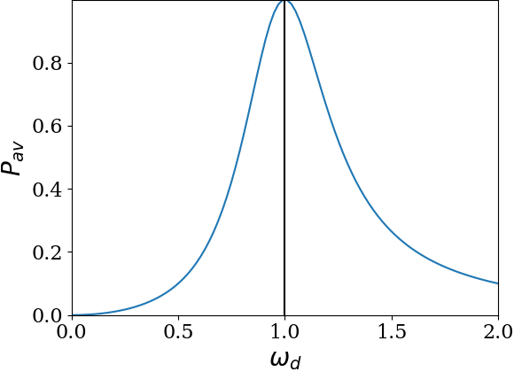
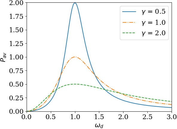
\amp P_\text{av}(\omega_d) = \frac{F_0^2}{2\, m\, \gamma} \end{align*}
This gives
\begin{equation*} \omega_d^4 - \left( 2\omega_0^2 + \gamma^2\right)\,\omega_d^2 + \omega_0^4 = 0. \end{equation*}
Let \(x=\omega_d^2\) and solve the quadratic equation for \(x\text{.}\)
\begin{align*} \omega_d^2 \amp = \frac{1}{2} \left[ \left( 2\omega_0^2 + \gamma^2 \right) \pm \sqrt{ \left( 2\omega_0^2 + \gamma^2 \right)^2 - 4 \omega_0^4 } \right] \\ \amp = \omega_0^2 + \frac{1}{2} \gamma^2 \pm \omega_0\gamma \sqrt{ 1 + \frac{\gamma^2}{4 \omega_0^2} } \\ \amp \approx \omega_0^2 \pm \omega_0\gamma \left( 1 \right) \ \ \ \text{since } (\gamma/\omega_0) \ll 1. \end{align*}
Now, we take square root to get
\begin{equation*} \omega_d = \pm \sqrt{ \omega_0^2 \pm \omega_0\gamma }. \end{equation*}
Looking at the positive root (negative root gives same range.) we have
\begin{align*} \omega_d \amp = \sqrt{ \omega_0^2 \pm \omega_0\gamma } \\ \amp = \omega_0 \left( 1 \pm \frac{\gamma}{\omega_0} \right)^{1/2}\\ \amp \approx \omega_0 \left( 1 \pm \frac{1}{2}\,\frac{\gamma}{\omega_0} \right) \\ \amp = \omega_0 \pm \frac{1}{2}\,\gamma \end{align*}
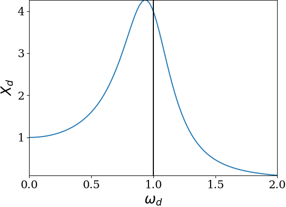
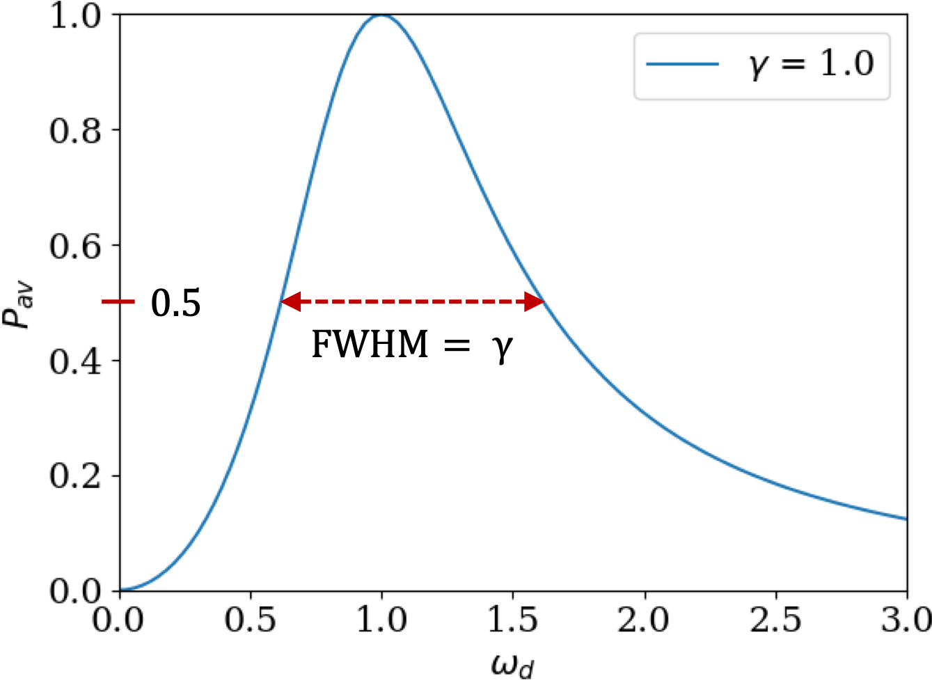
Thus, the value of \(\omega_d\) at half maximum has two values around the peak; let’s call them left and right values.
\begin{align*} \amp \left( \omega_d \right)_\text{left} = \omega_0 - \frac{\gamma}{2}.\\ \amp \left( \omega_d \right)_\text{right} = \omega_0 + \frac{\gamma}{2}. \end{align*}
Hence, the width at half maximum is
\begin{equation*} \text{FWHM} = \left( \omega_d\right )_\text{right} - \left(\omega_d \right)_\text{left} = \gamma. \end{equation*}

Exercises 13.10.8 Exercises

1. Resonance of an Underdamped Driven Oscillator.

A block of mass \(0.2\text{ kg}\) is hung from a spring of spring constant \(100\text{ N/m}\text{.}\) The block is subject to a viscous drag, \(F_{\text{visc}} = - b v\text{,}\) with \(b = 3\text{ N.s/m}\text{.}\) A driving force \(F_d = F_0\,\cos(\omega_d t)\text{,}\) with \(F_0 = 5\text{ N}\) and \(\omega_d = 20\text{ rad/s}\text{,}\) also acts on the block.
(a) What is the amplitude of oscillations of the block in the steady state?
(b) If frequency \(\omega_d \) is varied, at what value of \(\omega_d \) is the steady state amplitude largest?
(c) If frequency \(\omega_d \) is varied, at what value of \(\omega_d \) average power delivered by the driving force is the largest?
Hint.
(a) Use formula for \(X_d\text{.}\) (b) Use resonance of amplitude. (c) Use resonance of average power.
Answer.
(a) \(0.08\text{ m}\text{,}\) (b) \(16.6\text{ sec}^{-1} \text{,}\) (c) \(22.36\text{ sec}^{-1}\text{.}\)
Solution 1. (a)
(a) We just plug in the numbers in the formula for \(X_d\text{.}\) But first we find the values of the effective parameters.
\begin{align*} \omega \amp = \sqrt{ \dfrac{k}{m} } = \sqrt{ \dfrac{100}{0.2} } = 22.36\text{ sec}^{-1},\\ \gamma \amp = \dfrac{b}{m} = \dfrac{3}{0.2} =15\text{ sec}^{-1}, \end{align*}
Using these in the formulas for \(X_d\) we get
\begin{equation*} X_d = \dfrac{5/0.2}{\sqrt{ ( 22.36^2 - 20^2 )^2 + ( 20\times 15 )^2 }} = 0.08\text{ m}. \end{equation*}
Solution 2. (b)
(b) We seek the value of \(\omega_{R,X_d} \text{.}\)
\begin{equation*} \omega_{R,X_d} = \sqrt{ \omega^2 - \gamma^2 } = \sqrt{ 22.36^2 - 15^2 }=16.6\text{ sec}^{-1}. \end{equation*}
Solution 3. (c)
(c) The resonance of average power occurs at angular frequency \(\omega = 22.36\text{ sec}^{-1}\text{.}\)

2. Phase at Resonance of an Underdamped Driven Oscillator.

An underdamped oscillator of mass \(m = 0.2\) kg with \(\beta = \frac{\omega_0}{10}=2\) rad/sec is driven by a harmonic driving force \(\vec F_{d}\text{.}\) The oscillator oscillates in \(x\)-axis. The driving force has the following \(x\)-component: \(F_{x} = (5N)\cos(\omega_d t)\text{.}\) (a) Find the phase difference between the driving force and the displacement, if the driving frequency is equal to (i) \(0.1\omega_R\text{,}\) (ii) \(0.9\omega_R\text{,}\) or (iii) \(1.1\omega_R\text{.}\) (b) At what frequency would the phase difference be \(-\frac{\pi}{4}\) radian?
Solution 1. a
This problem uses formulas for the phase lag \(\delta\) given in the text.
\begin{equation*} \tan\delta = \frac{2\beta\omega_d}{\omega_0^2 - \omega_d^2}. \end{equation*}
The phase lag \(\delta\) is defined so that while the argument of the cosine in the driving frequency is \((\omega_d t)\) the argument for the \(x\) is \((\omega_d t-\delta)\text{.}\) The phase lag at resonance frequency is
\begin{equation*} \tan\delta_R = \frac{2\beta\omega_R}{\omega_0^2 - \omega_R^2} = \frac{1}{\beta}\sqrt{\omega_0^2 - 2\beta^2} = 9.9. \end{equation*}
This gives \(\delta_R = 84^{\circ}\text{.}\) The phase at the three frequencies in the question are obtained by plugging in the corresponding values of the frequencies in the expression for \(\tan\delta\text{:}\) (i) \(\omega_d = 1.98\) rad/s, (ii) \(\omega_d = 17.8\) rad/s, and (iii) \(\omega_d = 21.8\) rad/s. We find the (i) \(\delta = 1.15^{\circ}\text{,}\) (ii) \(\delta = 40.8^{\circ}\text{,}\) and (iii) \(\delta = -49.5^{\circ}\text{.}\)
Solution 2. b
Setting \(\delta = \pi/4\) we solve for \(\omega_d\) noting that \(\omega_d\) would be positive gives
\begin{equation*} \omega_d = -\beta + \sqrt{\beta^2 + \omega_0^2} = 18.1\ \textrm{rad/s}. \end{equation*}

3. Quality of a Damped Driven Oscillator from Information about Resonance.

A harmonically driven lightly damped oscillator has a resonance frequency of average power at \(100\text{ Hz}\text{.}\) The width of the power curve is \(\pi\text{ s}^{-1}\text{.}\) Find the quality of the oscillator.
Hint.
Use properties of the power resonance curve.
Answer.
\(200\text{.}\)
Solution.
Since width of power resonance curve is equal to the damping parameter \(\gamma\text{.}\)
\begin{equation*} \omega = 2\pi\times 100\text{ Hz} = 200\pi\text{ s}^{-1},\ \ \gamma = \pi\text{ s}^{-1}. \end{equation*}
Therefore,
\begin{equation*} Q = \frac{\omega}{\gamma} = 200. \end{equation*}

4. An Extensive Exercise on Driven Damped Oscillator.

A block of mass 300 grams is attached to a spring of spring constant \(100\) N/m. The block moves in an environment that damps its motion. The damping force is proportional to the speed of motion of the mass with the constant of proportionality given as \(0.1\) N.s/m. A sinusoidal driving force acts on the block with amplitude \(10\) N and a variable frequency. Find the following.
  1. The natural frequency of the oscillator
  2. The type of damping of the oscillator - under, over or critical
  3. The \(Q\) factor of the oscillator
  4. The resonance frequency of the oscillator
  5. The amplitude and phase of the oscillator in the steady state when the frequency of the driving force are: i. 0.25 \(\omega_R\text{,}\) ii. 0.5 \(\omega_R\text{,}\) iii. 0.75 \(\omega_R\text{,}\) iv. \(\omega_R\text{,}\) v. 1.25 \(\omega_R\text{,}\) vi. 1.5 \(\omega_R\text{,}\) vii. 1.75 \(\omega_R\text{,}\) viii. 10 \(\omega_R\text{.}\)
Solution 1. a
We start with listing the given values. \(m = 0.3\) kg, \(k = 100\) N/m, \(b = 0.1\) N.s/m, \(F_0 = 10\) N.
The natural frequency refers to \(\omega_0 = \sqrt{k/m}\text{.}\) Putting in given data we get \(\omega_0 = 18.3\) rad/s.
Solution 2. b
To decide on the type of damping we evaluate \(\beta\text{.}\) For the given values, \(\beta = b/2m = 0.167\) rad/s. Since \(\omega_0>\beta\text{,}\) the damping is under-damping.
Solution 3. c
\(Q = \omega_0/2\beta = 54.8\text{.}\)
Solution 4. d
The resonance of the amplitude of oscillations occurs at \(\omega_R = \sqrt{\omega_0^2 - 2\beta^2} \approx 18.3\) rad/s.
Solution 5. e
Use the following formulas to compute the amplitudes and phase lags at different \(\omega_d\) given.
\begin{align*} \amp A = \frac{D}{\sqrt{(\omega_0^2 - \omega_d^2)^2 +(2\beta\omega_d)^2}}.\\ \amp \tan\delta = \frac{2\beta\omega_d}{\omega_0^2 - \omega_d^2}. \end{align*}

5. Practice Definitions in Driven Damped Harmonic Oscillator.

Consider a one-dimensional damped oscillator of mass \(m = 0.5\) kg, \(\omega_0\) = 10 rad/sec, and \(\beta= 1\) rad/sec. Suppose the oscillator can oscillate along the \(x\)-axis. A sinusoidal force with the \(x\) component \(F_x = 100\ \textrm{N}\cos(\omega t)\) acts on the oscillator.
  1. What should be the condition on time \(t\) so that the steady state for the oscillator can be assumed?
  2. Suppose the steady state has been reached and the displacement of the oscillator can be written as \(x = A_c \cos(\omega t) + A_s \sin(\omega t)\text{.}\) Find the amplitudes \(A_c\) and \(A_s\) as a function of driving frequency \(\omega\text{.}\)
  3. Find the amplitude of the steady sate oscillations.
  4. Find the phase lag?
  5. What is the expression for the instantaneous power of the driving force?
  6. Find the average power as a function of driving frequency.
  7. At what frequency is the power maximum?
  8. At what frequency is the amplitude of the oscillator’s motion maximum?
  9. What is the width at half height of the power versus driving frequency plot?
Solution.
Let us start with listing the given quantities.
\begin{equation*} m = 0.5\,\text{kg},\ \ \omega_0 = 10\,\text{rad/sec},\ \ \beta = 1.0\,\text{rad/sec},\ \ F_0 = 100\,\text{N}. \end{equation*}
  1. Steady state when \(t>>1/\beta\text{.}\) This means that we need to wait for \(t>>1\) sec before assuming the steady state condition for the given oscillator.
  2. Left as an exercise for the student.
  3. Amplitude of the steady state solution is related to the \(A_c\) and \(A_s\) and has been given in the textbook.
    \begin{equation*} A = \frac{D}{\sqrt{(\omega_0^2 - \omega^2)^2 +(2\beta\omega)^2}}. \end{equation*}
    Here \(D = F_0/m\text{.}\)
  4. The phase lag \(\delta\) will be given by
    \begin{equation*} \tan\delta = \frac{2\beta\omega}{\omega_0^2 - \omega^2}. \end{equation*}
  5. The instantaneous power of the driving force is
    \begin{equation*} P(t) = \vec F_d \cdot \vec v = F_x v_x. \end{equation*}
    With \(x = A\cos(\omega t-\delta)\) and \(F_x = F_0\cos(\omega t)\) we get
    \begin{equation*} P(t) = -\omega A F_0 \cos(\omega t)\cos(\omega t-\delta). \end{equation*}
    If you used \(x(t) = A_c \cos(\omega t) + A_s \sin(\omega t)\text{,}\) then you would get
    \begin{equation*} P(t) = \omega F_0 \cos(\omega t)\left[ -A_c\sin(\omega t) + A_s\cos(\omega t) \right]. \end{equation*}
  6. The average power will be
    \begin{equation*} P_{\textrm{ave}} = \frac{1}{2}\omega F_0 A_s. \end{equation*}
    In terms of the formula using the amplitude \(A\) we get
    \begin{equation*} P_{\textrm{ave}} = \frac{1}{2}\omega F_0 A\sin\delta. \end{equation*}
  7. Power is maximum at its resonance frequency, which occurs at \(\omega = \omega_0\text{.}\)
  8. The maximum amplitude occurs at its resonance frequency which occurs at \(\omega = \sqrt{\omega_0^2-2\beta^2}\text{.}\)
  9. Setting the general expression for \(P_{\textrm{ave}}\) in ????.