Resistors, capacitors, and inductors are called
passive elements of a circuit while EMF source is called the
active element. In the absence of external magnetic field through the surface of a circuit, Faraday’s law simplifies to a rule similar to Kirchhoff’s voltage rule, which we might call pseudo-Kirchhoff’s voltage law, as long as we take care of back-emf voltage drop due to inductance of the circuit as we will see below. If you place the AC circuit in an external dynamic magnetic field whose flux may be varying, then you better include the rate of magnetic flux also as required by Farady’s law.
In this section, we will work out formulas for voltage drops across each element to be used in the pseudo-Kirchhoff’s rule. We will find that voltage across each element and current through them will depend on the frequency of the AC circuit. Furthermore, we need phase constant diferences between current and voltage for all passive elements.
Voltage Drop Across a Resitor
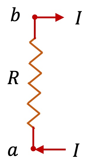
Suppose current \(I\) passes through a resistor of resistance \(R\text{.}\) Then, voltage drop across the resistor, denoted as \(V_R\) will be given by Ohm’s law.
\begin{equation*}
V_R = R\, I(t).
\end{equation*}
For an AC current \(I(t) = I_0\, \cos(\omega t + \phi_I)\text{,}\) we will get
\begin{equation*}
V_R(t) = R\, I_0 \cos(\omega t + \phi_I).
\end{equation*}
If we write \(V_R(t)\) in terms of its own magnitude and phase constant, i.e.,
\begin{equation*}
V_R(t) =V_{R0}\, \cos(\omega t + \phi_V),
\end{equation*}
then, we find that current through a resistor and voltage across resistor are in-phase, i.e., their phases are same.
\begin{equation}
\phi_V = \phi_I,\quad V_{R0} = R\, I_0 .\tag{41.5}
\end{equation}
Important thing to note here is that voltage and current amplitudes across a resistor here have same relation as in the DC circuit case and they are in sync with each other.
Voltage Drop Across an Inductor
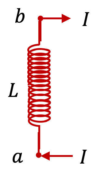
Suppose current
\(I\) passes through an inductor of self-inductance
\(L\text{.}\) When current is increasing, then there is a
back emf, which can be interpreted as a voltage drop across the inductor and when current is decreasing, there is a forward emf, which can be interprested as additional voltage source.
Interpreting back emf and forward emf as voltages, we denote them by \(V_L\text{.}\) The relation of \(V_L\) with current \(I\) is not as simple as Ohm’s law for resistance.
\begin{equation*}
V_L = L\,\dfrac{dI}{dt}.
\end{equation*}
For an AC current with \(I(t) = I_0\, \cos(\omega t + \phi_I)\text{,}\) we will get
\begin{equation*}
V_L(t) = - \omega L\, I_0\, \sin(\omega t + \phi_I).
\end{equation*}
We need to express \(V_L\) as cosine since we want to compare its phase to that of current \(I\text{,}\) which we are writing in cosine. When we change from sine to cosine, we will want to absorb the sign also. Therefore, \(V_L\) is
\begin{equation*}
V_L(t) = \omega\, L\, I_0\, \cos(\omega t + \phi_I + \frac{\pi}{2} ).
\end{equation*}
If we write \(V_L(t)\) in terms of its own magnitude and phase constant, i.e.,
\begin{equation}
V_L(t) =V_{L0}\, \cos(\omega t + \phi_V),\tag{41.6}
\end{equation}
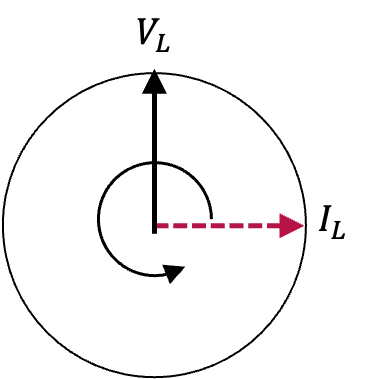
then, we find that current through an inductor and voltage across the inductor are not in-phase, but voltage is \(\dfrac{\pi}{2}\) radians or \(90^\circ\) is ahead of the current.
\begin{equation}
\phi_V = \phi_I + \dfrac{\pi}{2},\quad V_{L0} = \omega L I_0.\tag{41.7}
\end{equation}
From the amplitude relation \(V_{L0} = \omega L I_0 \text{,}\) we see that inductor provides a frequency-dependent “resistance”. We call this resistance by another name, inductive reactance and denote it by \(X_L\text{.}\)
\begin{equation}
X_L = \omega\, L.\tag{41.8}
\end{equation}
The phase relation in Eq.
(41.7) shows that, across an inductor,
\(\phi_V \gt \phi_I\text{.}\) We say that, across an inductor,
voltage leads current.
We can visualize the phase relation between voltage across the inductor and current through the inductor by thinking of them as arrows rotating at the same rate (both rotating
\(\omega\,t\) angle in time
\(t\)) in a plane whose angle is the phase as in
Figure 41.8.
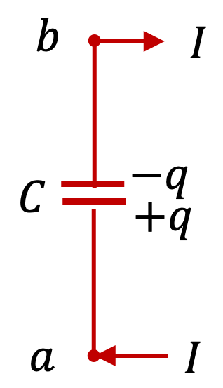
Voltage Drop Across a Capacitor
\(I\)\(C\text{,}\)\(q\)
Suppose \(q=0\) at \(t=0\text{,}\) then, charge at instant \(t\) will be
\begin{equation*}
q(t) = \int_0^t I(t) dt.
\end{equation*}
Voltage across a capacitor, denoted by \(V_C\text{,}\) will be given by the capacitor equation.
\begin{equation*}
V_C = \dfrac{1}{C}\, q.
\end{equation*}
Therefore, we will have
\begin{equation}
V_C = \dfrac{1}{C}\, \int_0^t I(t) dt\tag{41.9}
\end{equation}
For an AC current with \(I(t) = I_0\, \cos(\omega t + \phi_I)\text{,}\) we will get
\begin{equation}
V_C(t) = \dfrac{1}{\omega C}\, I_0 \sin(\omega t + \phi_I).\tag{41.10}
\end{equation}
We need to express \(V_C\) as cosine since we want to compare its phase to that of current \(I\text{,}\) which we are writing in cosine. Therefore, \(V_C\) is
\begin{equation}
V_C(t) = \dfrac{1}{\omega C}\, I_0 \cos(\omega t + \phi_I - \frac{\pi}{2} ).\tag{41.11}
\end{equation}
If we write \(V_C(t)\) in terms of its own magnitude and phase constant, i.e.,
\begin{equation}
V_C(t) = V_{C0} \cos(\omega t + \phi_V),\tag{41.12}
\end{equation}
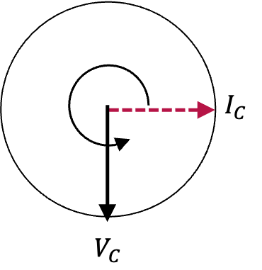
then, we find that current into a capacitor and voltage across the capacitor are not in-phase, but voltage is \(\dfrac{\pi}{2}\) radians or \(90^\circ\) is behind the current.
\begin{equation}
\phi_V = \phi_I - \dfrac{\pi}{2},\ \ \ V_{C0} = \dfrac{1}{\omega C}\, I_0.\tag{41.13}
\end{equation}
From the amplitude relation \(V_{C0} = \dfrac{1}{\omega C}\, I_0 \text{,}\) we see that capacitor provides a frequency-dependent resistance. We call this resistance by another name, capacitative reactance and denote it by \(X_C\text{.}\)
\begin{equation}
X_C = \dfrac{1}{\omega C}.\tag{41.14}
\end{equation}
The phase relation in Eq.
(41.13) shows that, across a capacitor,
\(\phi_I \gt \phi_C\text{.}\) We say that, in the case of a capacitor,
current leads voltage.
We can visualize the phase relation between voltage across the capacitor and current into the capacitor by thinking of them as arrows rotating at the same rate (both rotating
\(\omega\,t\) angle in time
\(t\)) in a plane whose angle is the phase as in
Figure 41.10.
There is a cool mnemonic to remember the phase relations between the EMF and current for inductor and capcitor: “ELI the ICE man”. The ELI stands for in the case of inductor
\((L)\text{,}\) EMF
\(E\) leads current
\(I\) and the ICE stands for, in the case of capacitor
\((C)\text{,}\) current
\(I\) leads EMF
\(E\text{.}\)