Faraday’s Flux Rule and Lenz’s Law

Section 38.3 Faraday’s Flux Rule and Lenz’s Law

Various experiments of Faraday show that an electricity is induced in a circuit when there is a changing magnetic field or if the loop is moving in a magnetic field. These effects are collectively called the electromagnetic induction.

Faraday reasoned that the induced current in the loop must be due to some driving force in the wire, as is the case with any current in a wire. However, different experiments of Faraday appear to imply different mechanisms at work in different situations. We find two sources for the induced EMF in these experiments.

Subsection 38.3.1 Moving Conductors

For instance, when the magnet is fixed and the loop is moving, the current may be said to arise from the magnetic force $\vec F_m = q \vec v\times \vec B$ on the conduction electrons of the wire. The conduction electrons are guided along the loop by the cumulative influence of this magnetic force. The induced EMF in this circuit will be equal to the line integral of the magnetic force per unit charge along the circuit.

\begin{equation} \left|\mathcal{E}_\textrm{{ind}}\right| = \left|\oint \left( \vec v \times \vec B \right) \cdot d\vec l \right|\ \ \textrm{(Moving conductor.)}\tag{38.4} \end{equation}

Consider a moving cross-bar on a U-shaped metal placed in a uniform magnetic field as shown in Figure 38.12. When you pull on the bar to the right so that the bar slides with a constant velocity, an EMF will be induced in the circuit which will be equal to the line integral given in Eq. (38.4).

Doing the line integral in the loop a-b-c-d-a we get zero for all parts except a-b part since $B=0$ in those parts.

\begin{align} \left|\mathcal{E}_\textrm{{ind}}\right| \amp = \left|\int_{\textrm{abcda}} \left( \vec v \times \vec B \right) \cdot d\vec l\right| \notag\\ \amp = 0 + \left|\int_{\textrm{ab}} \left( \vec v \times \vec B \right) \cdot d\vec l\right|\ (\text{since } v=0 \text{ in other parts.})\notag\\ \amp = vB w.\quad (\text{since }\vec v \times \vec B = v\,B,\, \text{a constant}) \tag{38.5} \end{align}

That is, an EMF is induced in a circuit as a result of movement of a part of the circuit in a magnetic field.

An intriguing feature of this result is that the line integral of $\vec v\times \vec B$ is actually equal to the rate at which magnetic flux through the loop abcda of the circuit changes since the area A enclosed by the loop is changing.

\begin{equation*} \left|\int_{\textrm{abcda}} \left( \vec v \times \vec B \right) \cdot d\vec l\right| = \left| B \frac{d A}{dt} \right|= \frac{d \Phi_B}{d t}\ \ \textrm{(since B is constant.)} \end{equation*}

This important “coincidence” turns out to be a special case of the Faraday flux rule to be discussed below.

Subsection 38.3.2 Changing Magnetic Field

When the wire is held fixed and the magnet is moving, there is no $q \vec v\times \vec B$ force on the charges. Faraday found that the induced EMF in these circuits is due a new effect. He found that when the circuit is not moving but instead the magnetic field through the space of the circuit is varying, then the induced EMF is proportional to the rate of change of the magnetic field.

\begin{equation} \left| \mathcal{E}_\textrm{ind} \right| \propto \left| \frac{dB}{dt}\right|\ \ \ \textrm{ ( Fixed circuit, Fixed orientation.) }\tag{38.6} \end{equation}

This kind of experiment is easily done in experiments like Figure 38.4 where the magnetic field through the loop can be varied by turning the switch for the current in the solenoid on/off and/or moving the solenoid while holding the loop #2 fixed in position.

It is possible to state the two effects that lead to induced EMF in a loop of wire, viz. one due to the changing magnetic field and the other due to the motion of the wire into one relation. This relation is due to Faraday and is called the Faraday flux rule. The induced effect in places where there is no clear loop of wire, e.g. in a moving rod or a rotating disk the induced EMF is understood in terms of the magnetic force $\vec v\times \vec B$ on mobile charges in moving conductors.

Subsection 38.3.3 Faraday’s Flux Rule

Faraday explained all of his experiments by a simple rule, often referred to as Faraday’s flux rule. It states that induced EMF in a loop is equal to the rate at which magnetic flux through the loop is changing. Sometimes this rule is also referred to as Faraday’s law - we will reserve that phrase for a more general result to be described in Section 38.7.

Let us denote induced EMF by $\mathcal{E}_\text{ind}$ rather than symbol $V$ since we are dealing with dynamical quantity as opposed to static quantity of a voltage of a battery. According to Faraday’s flux rule, average induced EMF during interval $t$ to $t+\Delta t$ is given by the rate of change of magnetic flux.

\begin{equation} \mathcal{E}_\text{ind,ave} = - \dfrac{\Delta \Phi_B}{\Delta t}.\tag{38.7} \end{equation}

You can see that the unit of $\Delta \Phi_B / \Delta t$ is actually volts, same as the unit of battery voltage. Thus, if at some instant, $\Delta \Phi_B / \Delta t$ was $12\text{ V}$ (not $\text{V/s}\text{,}$ but rather $\text{T.m}^2/\text{s}$), then, the closed loop will act as if a $12\text{ V}$ “fictitious” battery was inserted in the loop. We will see examples of its applications below.

Subsubsection 38.3.3.1 Case of Uniform Magnetic Field

Recall that if we have a uniform magnetic field $\vec B\text{,}$ whether changing in time or not, its flux through a flat surface of area $A$ which is oriented so that the normal to the area makes an angle $\theta$ with $\vec B\text{,}$ then, magnetic flux through a loop around the edges of the flat surface is given by

\begin{equation*} \Phi_{B} = B\, A\, \cos\,\theta. \end{equation*}

By takng its time derivative we can immediately know various ways flux can change.

\begin{equation*} \frac{d\Phi_B}{dt} = \frac{dB}{dt}\,A\, \cos\,\theta + B\,\frac{dA}{dt}\,\cos\,\theta + (-1)\, B\, A\, \sin\,\theta\,\frac{d\theta}{dt}. \end{equation*}

Therefore, a change in magnetic flux can occur in three ways:

$\Delta \Phi_B$ due to changing $B\text{,}$ i.e, changing strength of $\vec B\text{,}$ which we indicate by adding $B$ to the subscript.

\begin{equation*} \Delta \Phi_{B,B} = (A \cos\,\theta )\Delta B, \end{equation*}
$\Delta \Phi_B$ due to changing $A\text{,}$ i.e, changing area in the loop through which field lines may go through,

\begin{equation*} \Delta \Phi_{B,A} = (B \cos\,\theta )\Delta A, \end{equation*}
$\Delta \Phi_B$ due to changing $\theta\text{,}$ i.e, relative orientation of $\vec B$ and area.

\begin{equation*} \Delta \Phi_{B,\theta} = -(B A \sin\,\theta )\Delta \theta, \end{equation*}

when you are looking at changing orientation with time.

Pooling the three types of contributions you will get the net change in flux in time $\Delta t\text{.}$

\begin{equation} \Delta \Phi_B = \Delta \Phi_{B,B} + \Delta \Phi_{B,A} + \Delta \Phi_{B,\theta}.\tag{38.8} \end{equation}

Therefore, in the case of uniform magnetic field through a flat area, induced EMF will come from three sources.

\begin{equation} \mathcal{E}_\text{ind,ave} = - \dfrac{\Delta \Phi_{B,B}}{\Delta t} -\dfrac{\Delta \Phi_{B,A}}{\Delta t} - \dfrac{\Delta \Phi_{B,\theta}}{\Delta t}.\tag{38.9} \end{equation}

Faraday’s experiments described in Section 38.1 illustrate these mechanisms by which flux can change in a closed loop.

Direction of Induced Current. We will see below in Subsection 38.3.5 that Lenz’s law is an easier way to glean the direction of induced current, but here we make the point that minus sign in Eq. (38.7) tells us the direction of the induced EMF, itself, which is the direction of the induced current.

Minus sign in Eq. (38.7) gives us the direction of induced current when we use right-hand rule to assign direction to the area of the loop as illustrated in Figure 38.13. If $\mathcal{E}_\text{ind,ave}$ is positive, then induced current will be in the direction of the area vector and if $\mathcal{E}_\text{ind,ave}$ is negative, then induced current is in the opposite direction.

Magnitude of Induced Current. Let $\mathcal{E}_\text{ind}$ be the induced EMF in a loop of wire that has resistance $R\text{,}$ then by Ohm’s law we would get induced current $I_\text{ind}\text{.}$

\begin{equation} I_\text{ind} = \dfrac{1}{R}\,\mathcal{E}_\text{ind}.\tag{38.10} \end{equation}

So, how is $\mathcal{E}_\text{ind}$ related to moving conductor, moving magnet, or changing magnetic field? We will work formulas out in particular situations below and then give a complete answer in the end.

Subsection 38.3.4 Flux Rule and Stacking Loops

Faraday used stacked coils to enhance the induced EMF in the loop. A long wire is twisted into coils and the ends of the wire are connected to complete the loop. We can now understand why coils enhance the electromagnetic effect.

Consider two circuits labelled $\mathcal{C}_1$ and $\mathcal{C}_2$ in Figure 38.14 which are made of identical material and have the same size loops. In the circuit $\mathcal{C}_1$ there is only one loop and in the circuit $\mathcal{C}_2$ there are four loops which are connected so that the induced current would flow parallel in all the loops. Note that the wire will have to be twisted to connect the ends so that current flows in the same direction in all the loops.

Figure 38.14. Varying magnetic field induces four times as much EMF as in circuit $\mathcal{C}_2$ as in circuit $\mathcal{C}_1$ and hence four times as much current.

Suppose we place circuit $\mathcal{C}_2$ in an external magnetic field and then we vary the strength of the field.

Now, we ask: how do various quantities in the two circuits compare? In particular, we compare the rates of the change magnetic fluxes and the induced EMFs in the two circuits. Let us use superscripts $(1)$ and $(2)$ for the quantities in the two circuits.

We see that a simple surface can be attached to calculate the magnetic flux through the one-loop circuit $\mathcal{C}_1\text{,}$ but no simple surface can be attached to all the wires of circuit $\mathcal{C}_2$ due to the connecting wires on the side. In Figure 38.14, I have highlighted only the loop areas and omitted other areas around the loop that would be need for all areas enclosed by the entire circuit. These other areas are negligible in our case and it is okay to ignore them. With this assumption, we see that the magnetic flux through $\mathcal{C}_2$ is four times the magnetic flux through $\mathcal{C}_1\text{.}$

\begin{equation*} \left|\Phi_B^{(2)}\right| \approx 4\times \left|\Phi_B^{(1)}\right| \end{equation*}

We will now ignore the small error we make in neglecting the extra surface on the side of the loops and will write the relations as an equality below. Thus, the rate of change of the magnetic flux through $\mathcal{C}_2$ is four times that through $\mathcal{C}_1\text{.}$

\begin{equation*} \left|\dfrac{d\Phi_B^{(2)}}{dt} \right|= 4\times \left|\dfrac{d\Phi_B^{(1)}}{dt}\right|, \end{equation*}

which implies that the induced EMF in $\mathcal{C}_2$ would be four times that in $\mathcal{C}_1$

\begin{equation*} \mathcal{E}^{(2)} = 4\times \mathcal{E}^{(1)} \end{equation*}

Subsection 38.3.5 Lenz’s Law

When you examine the direction of the induced magnetic field by the induced current and compare it with the direction of the external magnetic field, you notice the following observation, known as Lens’s law.

The flux of the magnetic field generated by the induced current always opposes the change in the magnetic flux through the loop. Lenz explained this by claiming that each closed circuit has an inertia of magnetic flux and develops induced current to oppose any change in its state.

It is easy to figure out the direction of induced current by applying Lenz’s law. For instance, suppose external magnetic field was directed towards positive $z$ axis and it was increasing. In this case, the magnetic field of the induced current will be in the negative $z$ direction, as illustrated in Figure 38.15. On the other hand, if the magnetic field was decreasing, then, the magnetic field of the induced current will be in the positive $z$ direction.

From the required direction of the induced magnetic field, we can deduce the current that must have been induced by using Biot-avart’s right-hand rule.

Figure 38.15. As magnetic flux through the conducting loop in the direction into-the-page increases, the induced current in the loop develops, whose magnetic field must have the direction out-of-page, denoted by symbol $\bigotimes\text{,}$in the area of the loop to fight the increasing flux. To create magnetic field in $\bigotimes$ direction in the area of the loop, the induced current must be running counterclockwise by using Biot-Savart’s right-hand rule.

Subsection 38.3.6 Faraday’s Paradox

Faraday’s flux rule does not explain induced current in all stuations. For instance, Figure 38.16 shows an adaptation of Faraday’s disc problem in a practical setting, where you need to go beyond flux rule and include Lorentz force on moving electrons to explain the development of induced current.

In Figure 38.16, a conducting disc is connected to a galvanometer with one contact at the shaft and the other at the edge of the disc so that the contacts rub the metal shaft and the metal edge when the disc rotates. A magnet is fixed to provide a magnetic field perpendicular to the surface of the disc.

Figure 38.16. A metal disc is rotated in the presence of a fixed magnet. When the disc rotates, there is no change in magnetic flux through any choice of line on the disc to complete the loop through the galvanometer. Yet there is an induced current through the galvanometer. The EMF for the current through the galvanometer can be understood in terms of radially pointed Lorentz force, $q \vec v\times \vec B\text{,}$ on the moving conduction electrons at the points on the disc with non-zero magnetic field. Adapted from Feynman’s Lectures in Physics, Vol II.

First note that a unique circuit is not clear here since you can draw infinitely many lines on the disc between the contact at the edge and the contact at the shaft. The magnetic flux through any circuit you draw in space would not change with time. However, when the disc rotates a current is detected by the galvanometer.

A naive application of the flux rule gives us a contradiction here: the flux rule says that no flux change would mean no induced current. However, a closer look at the experimental setting shows that the magnetic force, $q\vec v\times\vec B\text{,}$ on the moving charges will cause a radial component of the velocity which will result in an overall drift of charges towards the shaft. The EMF in this setting develops neither from a changing magnetic field nor from a changing area of a loop or a changing orientation of a loop.

We can work out the induced EMF by Lorentz force as follows. Suppose electrons in the metal are moving with velocity $\vec v \text{,}$ then there would be magnetic force on conduction electrons along the wire, thus accelerating them perpendicular to their motion.

\begin{equation} \vec F_{m} = q \vec v \times \vec B.\tag{38.11} \end{equation}

This force on conduction electrons will cause drift motion in the conductor guided by the geometry of the conductor. Since accelerating electrons cannot leave the conductor, this results into an induced electric field in the conductor, which is equal to this force per unit charge.

\begin{equation} \vec E_\text{ind} = \dfrac{\vec F_{m} }{q} = \vec v_\perp \times \vec B.\tag{38.12} \end{equation}

Asssuming this field to have constant magnitude and flowing in the conducing loop of length $l\text{,}$ the EMF associated with this induced field will be

\begin{equation} \mathcal{E}_\text{ind} = - E l = - |\vec v_\perp \times \vec B| l .\tag{38.13} \end{equation}

Exercises 38.3.7 Exercises

1. Six Induced EMF and Lenz’s Law Exercises.

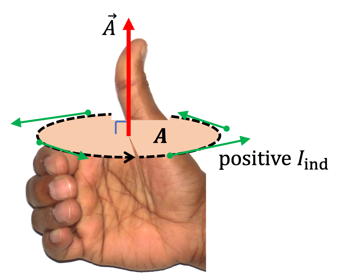
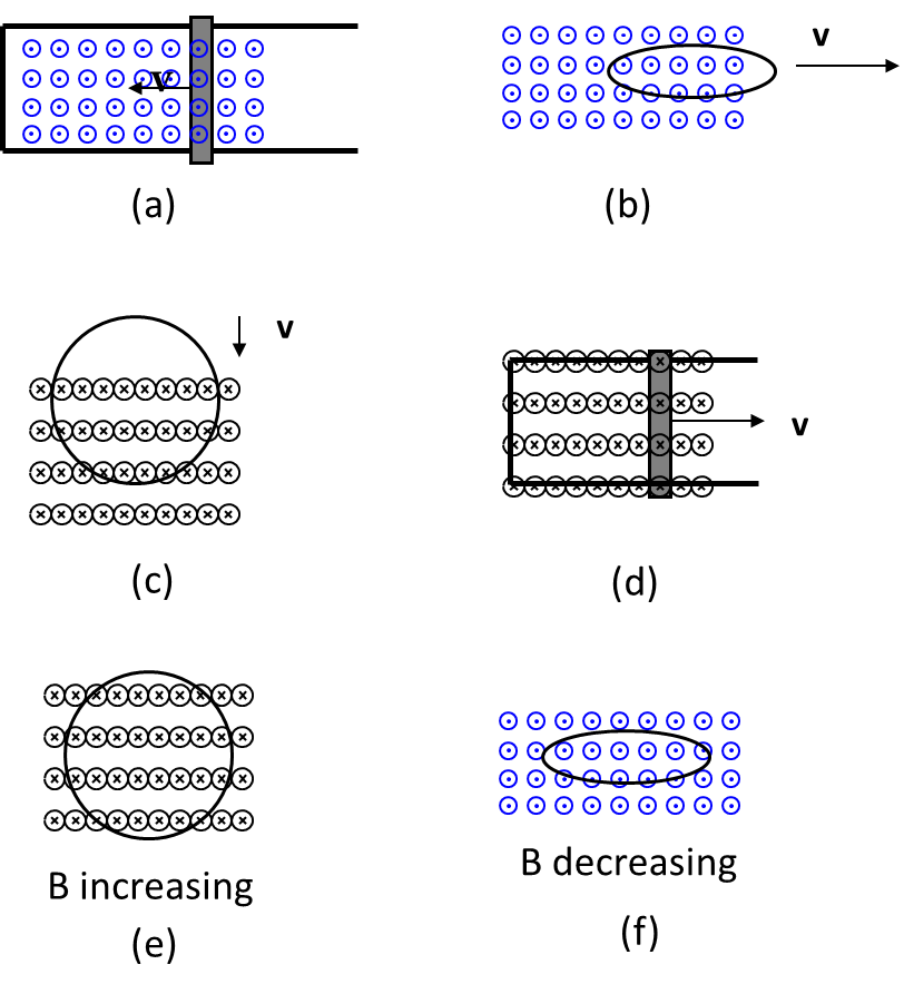
Use Lenz’s law to determine the direction of induced current in each case. Here a circle with a dot, $\bigodot$ represents magnetic field pointed out-of-page and a circle with an x, $\bigotimes$ for a magnetic field pointed in-the-page, and lines are conductors.

Hint.

Apply Lenz’s law.

Answer.

(a) up the rod, (b) counterclockwise, (c) clockwise, (d) counterclockwise, (e) counterclockwise, (f) counterclockwise.

Solution 1. (a)

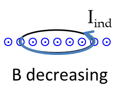
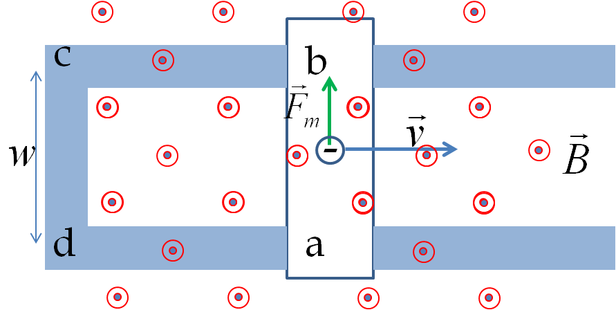
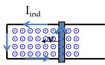
(a) Magnetic flux from magnetic field in the direction out-of page decreases inside the loop. Hence the induced current must create more of magnetic field in the out-of-page direction. Therefore the induced current will flow up in the rod.

Solution 2. (b)

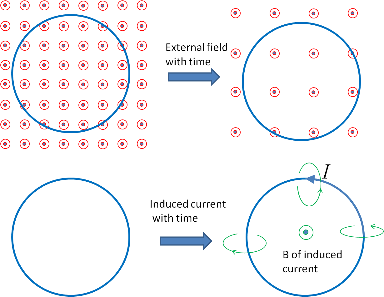
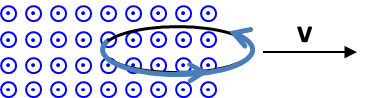
(b) Since the ring is leaving an area of magnetic field in the out-of page direction, the induced current in the ring must generate magnetic field in the out-of-page direction. Hence, induced current will be in the counterclockwise direction.

Solution 3. (c)

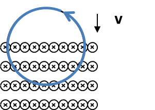
(c) The ring is moving so that magnetic flux from magnetic field in the in-the-page direction is increasing. Therefore the induce current will be creating magnetic field in the out-of-page direction so as to reduce the increase of in-the-page magnetic field. A current in the clockwise direction will be induced.

Solution 4. (d)

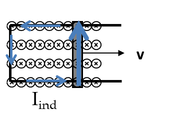
(d) As the bar moves, the loop encloses more of in-the-page magnetic field lines. Hence, the induced current will produce out-of-page magnetic field inside the space enclosed by the loop. Therefore, the induced current will run in a counterclockwise direction.

Solution 5. (e)

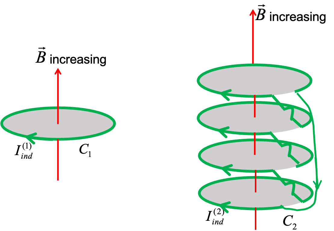
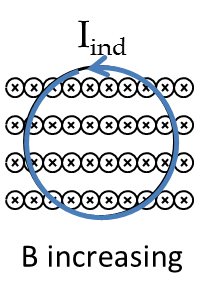
(e) When $B$ into the page is increasing, the magnetic flux through the ring for into-the-page will be increasing. The induced current will be in such a direction that the magnetic field of the induced current will be in the out-of page direction. Therefore, the direction of the induced current will be counterclockwise as shown.

Solution 6. (f)

(f) When $B$ out-of-page is decreasing, the magnetic flux through the ring for out-of-page will be decreasing. The induced current will be in such a direction that the magnetic field of the induced current will be in out-of page direction. Therefore, the direction of the induced current will be counterclockwise as shown.

2. Induced Current in Loop Between Poles of an Electromagnet.

A current is induced in a circular loop of radius $1.5\, \text{cm}$ between two poles of a horseshoe electromagnet when the current in the electromagnet is varied. The magnetic field in the area of the loop is perpendicular to the area and has a uniform magnitude. If the rate of change of magnetic field is $10\, \text{T/s}\text{,}$ find the magnitude and direction of the induced current if resistance of the loop is 25 $\Omega\text{.}$

Hint.

Use flux rule in combination with Lenz’s law.

Answer.

$2.83\times 10^{-4} \ \textrm{A}\text{.}$

Solution.

The magnitude of the induced current is found by dividing the induced EMF given by Faraday law.

\begin{equation*} I_{\textrm{ind}} = \dfrac{\left|d\Phi/dt \right|}{R_{\textrm{eq}}} = \dfrac{2\:\textrm{T/s}\times \pi (0.015\:\textrm{m})^2 }{5\:\Omega} = 2.83\times 10^{-4}\:\textrm{A}. \end{equation*}

The direction will be such that it will oppose the increase of magnetic flux as shown in Figure 38.23. The magnetic flux of the external field in the left to right direction is increasing. Therefore, induced magnetic field will be pointed to the left at points inside of the loop. The induced current will be in the direction shown.

Figure 38.23. Exercise 38.3.7.2 - direction of induced current.

3. Induced Current in a Circular Wire Surrounding a Solenoid from Varying Current in the Solenoid.

Current in a long solenoid of radius $3\, \text{cm}$ varies with time at a rate of $2\, \text{A/s}\text{.}$ A circular loop of wire of radius $5\, \text{cm}$ and resistance $2\,\Omega$ surrounds the solenoid. Find the electric current induced in the loop.

Hint.

Use loop rule.

Answer.

$7.1\, \mu\textrm{A}\text{.}$

Solution.

Note that even though there is no magnetic field at the site of the outer wire, there is a no-zero magnetic flux through the area of the loop which is changing in time. Hence, a current will be induced in the outer wire given by Faraday law.

\begin{align*} I_{\textrm{ind}} \amp = \dfrac{\mathcal{E}}{R_{\textrm{outer loop}}} \\ \amp = \dfrac{\mu_0\:n\:A_{\textrm{sol}}}{R_{\textrm{outer loop}}}\:\dfrac{\Delta I_{\textrm{sol}}}{\Delta t}, \end{align*}

where $A_{\textrm{sol}}$ is the area of cross-section of the solenoid and $I_{\textrm{sol}}$ is the current in the solenoid at time $t\text{.}$ Putting in the numerical values we obtain

\begin{equation*} I_{\textrm{ind}} = 7.1\times 10^{-6}\:\textrm{A}. \end{equation*}

4. (Calculus) Induced EMF in Two-loop Coil Surrounding a Solenoid with Sinusoidally Varying Current.

A long solenoid of radius a with n turns per unit length is carrying a time-dependent current $I(t) = I_0 \sin (\omega t)\text{,}$ where $I_0$ and $\omega$ are constants. The solenoid is surrounded by a wire of resistance $R$ that has two circular loops of radius $b$ with $b \gt a\text{.}$ Find the magnitude and direction of current induced in the outer loops at time $t=0\text{.}$

Hint.

Use flux rule to find the induced EMF first.

Answer.

$2\mu_0 \pi a^2 I_0 n\omega/R\text{.}$

Solution.

It is easier to calculate the magnetic flux of the magneitc field of the current in the solenoid through the outer loops since the magnetic field of the solenoid is constant.

\begin{equation*} \Phi_{\textrm{through outer loops}} = 2\times B_{\textrm{sol}}\times \pi a^2 = 2\times \mu_0\:n\:I_{\textrm{sol}}\times \pi a^2. \end{equation*}

Note the area over which the magnetic field of the solenoid is non-zero is only the inside of the solenoid. Since the current in the solenoid $I_{\textrm{sol}}$ is changing, the magnetic flux through the outer loops will change. The rate of change of this flux will induce an EMF in the outer loops.

\begin{equation*} \mathcal{E}_{\textrm{ind}} = \left| \dfrac{d\Phi}{dt}\right| = 2\pi\mu_0 a^2 I_0 n\omega|\cos\omega t|. \end{equation*}

Therefore, the induced current has the magnitude

\begin{equation*} I_{\textrm{ind}} = \dfrac{2\pi\mu_0 a^2 I_0 n\omega|\cos\omega t|}{R}. \end{equation*}

Since the current in the solenoid changes direction, thereby changing the direction of the magnetic flux, the induced current will also change direction with time.

5. (Calculus) Induced Current As a Result of a Varying Magnetic Field.

A circular loop of a copper wire of radius $a$ and resistance $R$ is placed in a uniform magnetic field whose direction is normal to the plane of the loop. While the direction of the magnetic field does not change with time, its magnitude changes with time according to $|\vec B(t)| = B_0 \exp{(-\alpha t)}\text{,}$ where $B_0$ is the magnitude at $t=0\text{.}$ Find the magnitude and direction of the induced current in the copper loop.

Hint.

Use $\mathcal{E} = -\dfrac{d\Phi_B}{dt}$ as magnitude first and then use Lenz’s law to get direction.

Answer.

$I = \dfrac{\mathcal{E}}{R} = \dfrac{\pi a^2 \alpha B_0}{R}\exp{(-\alpha t)}\text{,}$ counterclockwise.

Solution.

From Ohm’s law we know that the induced current will be equal to the induced EMF in the loop divided by the equivalent resistance of the loop of wire. To find the induced EMF, we need to evaluate the rate of change of the magnetic flux through the loop. Here the flux is changing due to the changing magnetic field whose analytic form has been provided. Therefore, we find the rate of change of the magnetic flux by taking the the time derivative of the magnetic flux.

Since the magnetic field is perpendicular to the area, the magnetic flux will be simply a product of the magnitude of the magnetic field and the area up to a sign. We will ignore the sign in our calculations of the magnitude of the induced current. The sign is related to the direction of the induced current, which we will obtain by applying Lenz’s law.

We will calculate the absolute value of the magnetic flux through the loop since we are gong to work with magnitudes first and we will find the direction of the induced current from Lenz’s law. The magnetic flux has the following magnitude here.

\begin{equation*} |\Phi_B| = \pi a^2B_0 \exp{(-\alpha t)}. \end{equation*}

The induced EMF in the loop will be

\begin{align*} \mathcal{E} \amp = \left| \dfrac{d\Phi_B}{dt}\right|\\ \amp =\pi a^2 \alpha B_0 \exp{(-\alpha t)} \end{align*}

Dividing the magnitude of the induced EMF by the equivalent resistance of the loop will give the magnitude of the induced current.

\begin{equation*} I = \dfrac{\mathcal{E}}{R} = \dfrac{\pi a^2 \alpha B_0}{R}\exp{(-\alpha t)}. \end{equation*}

Figure 38.25. Direction of the induced current by Lenz’s law. We use the fact that the magnetic field of the induced current opposes the change in the magnetic flux through the space of the loop. The top figures show that the magnetic flux for magnetic field pointed out-of-page is decreasing with time. The bottom figures show the induced current tending to compensate the loss of the magnetic flux by producing magnetic field in the direction in which the new magnetic field can mitigate the loss.

We now utilize Lenz’s law to determine the direction of the induced current. Let the direction of magnetic field be pointed up. The operational steps for the application of the Lenz’s law for this problem are shown in Figure 38.25. We start by noting that, since the magnitude of the magnetic field decreasing with time, the flux of the magnetic field of the type pointed-up would be decreasing with time. Therefore, according to the Lenz’s law, the magnetic flux of the magnetic field of the induced current must add to the magnetic flux of the pointed-up type field. That is, the magnetic field of the induced current should be pointed up at points inside the loop. This gives the direction of counter-clockwise for the induced current as looked from above as shown in Figure 38.25.

Prev Top Next