Electric Potential of Charged Conductors

Section 32.4 Electric Potential of Charged Conductors

Subsection 32.4.1 An Isolated Charged Metallic Sphere

Consider an isolated metallic sphere of radius \(R\) that has a total excess charge \(+q\) placed on it. The entire charge \(+q\) on the metallic sphere will end up at the surface as shown in Figure 32.24. Furthermore, as there are no other charges or bodies around, the charge distribution on the spherical surface will be spherically symmetric.

Aside Note: If there were other objects in the neighborhood of the metallic sphere, then the charges on the surface of the sphere will not necessarily be spherically symmetric - there will be more charges in certain direction than in other directions.

Since spherically distributed charge densiy has a spherical symmetry, we apply Gauss’s law to easily get the magnitude of electric field.

\begin{equation} E(r) = \begin{cases} 0 \amp r \lt R\\ \frac{1}{4\pi\epsilon_0}\,\frac{q}{r^2} \amp r \gt R \end{cases}\tag{32.5} \end{equation}

The direction of the electric field will be radially outward from the center of the sphere.

The electric field outside the charged spherical conductor is indistinguishable from that of a point charge \(+q\) placed at the center without the conductor present. The difference between the charged metal and a point charge occurs only at the space points inside the conductor: for a point charge placed at the center of the sphere, the electric field will not be zero at points of space occupied by the sphere, but for a conductor with the same amount of charge has a zero electric field at those points. However, there is no distinction at the outside points in space where \(r > R\text{,}\) and we can replace the isolated charged spherical conductor by a point charge at its center with impunity.

Electric Potential of a Charged Metallic Sphere

We find electric potential at a point P by integrating negative of the dot product of electric field with displacement from \(r=\infty\) (reference point) to the \(r=r\text{.}\) For a point P outside the conductor we will get

\begin{equation*} \phi(r_\text{out}) = -\int_\infty^{r_\text{out}}\, \frac{1}{4\pi\epsilon_0}\, \frac{dr}{r^2} = \frac{1}{4\pi\epsilon_0}\,\frac{q}{r_\text{out}} \end{equation*}

For a point P inside the sphere, the integral is nonzero upto the point \(r=R\) and zero when \(r \lt R\text{.}\) Therefore, we will get

\begin{equation*} \phi(r_\text{in}) = \frac{1}{4\pi\epsilon_0}\,\frac{q}{R}. \end{equation*}

With P outside, we get the same expression for potential as that of a point charge, but in the space inside the sphere, we get constant potential. These are sketched in Figure 32.25

\begin{equation*} \phi(r) = \begin{cases} \frac{1}{4\pi\epsilon_0}\,\frac{q}{R} \amp r \le R\\ \frac{1}{4\pi\epsilon_0}\,\frac{q}{r} \amp r \gt R \end{cases} \end{equation*}

Subsection 32.4.2 An Isolated Charged Long Metallic Wire

We have already worked out electric field of a charged wire of linear charge density \(\lambda\text{.}\) Using Gauss’s law for cylindrical symmetry, it was shown that electric field has the following magnitude at a ditance \(s\) from the wire.

\begin{equation*} E = \frac{\lambda}{2\pi\epsilon_0}\;\frac{1}{s}. \end{equation*}

In this case, the integral of the electric field will blow up if we choose the reference at \(s=\infty\) or \(s=0\text{.}\) So, we choose reference zero potential at a finite point, say \(s=s_\text{ref}\text{.}\) We can become more specific about the value of \(s_\text{ref}\) after doing the integral so that the formula for the potential is simplest.

\begin{equation*} \phi = -\int_{s_\text{ref}}^s\, \frac{\lambda}{2\pi\epsilon_0}\;\frac{ds}{s} = \frac{\lambda}{2\pi\epsilon_0}\;\ln\frac{s}{s_\text{ref}}. \end{equation*}

Now, if we choose \(s_\text{ref} = 1\) in the same unit as the unit of \(s\text{,}\) the formula will be simplest since \(\ln\,1 = 0\text{.}\) With this choice of the zero reference, the electric potential of the charges on a straight infinite wire at a distance \(s\) from the wire will be

\begin{equation*} \phi = - \frac{\lambda}{2\pi\epsilon_0}\;\ln\, s. \end{equation*}

Exercises 32.4.3 Exercises

1. Electric Field of Charged Metallic Spherical Shell Surrounding a Charged Metal Ball.

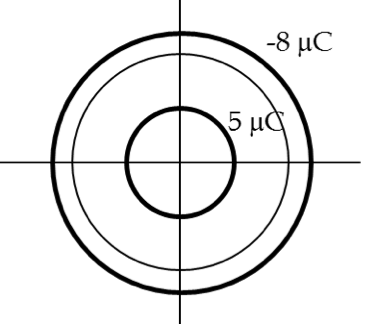
An aluminum spherical ball of radius \(4\text{ cm}\) is charged with \(5\ \mu\text{C}\) of charge. A copper spherical shell of inner radius \(6\text{ cm}\) and outer radius \(8\text{ cm}\) surrounds it. A total charge of \(-8\ \mu\text{C}\) is put on the copper shell.

(a) Find the electric field at all points in space including points inside the aluminum and copper shell when copper shell and aluminum sphere are concentric.

Figure 32.27. For Exercise 32.4.3.1 (a).

(b) Find electric potential at arbitrary point from the common center of the arrangement in part (a).

Hint.

(a) Use Gauss’s law. (b) Integrate the electric field from \(r=\infty\) to various points.

Answer.

See solution.

Solution 1. (a)

The given charge distributions have spherical symmetry. Therefore, a quick application of Gauss’s law yields the following for the electric field in various regions.

\begin{equation*} \vec E = \begin{cases} 0 \amp r\lt 4\:\text{cm}\\ \frac{1}{4\pi\epsilon_0}\:\frac{5\:\mu\text{C}}{r^2}\: \hat u_r \amp \ \ \ \ 4\:\text{cm} \lt r \lt 6\:\text{cm}\\ 0 \amp 6\:\text{cm} \lt r \lt 8\:\text{cm}\\ \frac{1}{4\pi\epsilon_0}\:\frac{-3\:\mu\text{C}}{r^2}\: \hat u_r \amp \ \ \ \ r > 8\:\text{cm} \end{cases} \end{equation*}

Solution 2. (b)

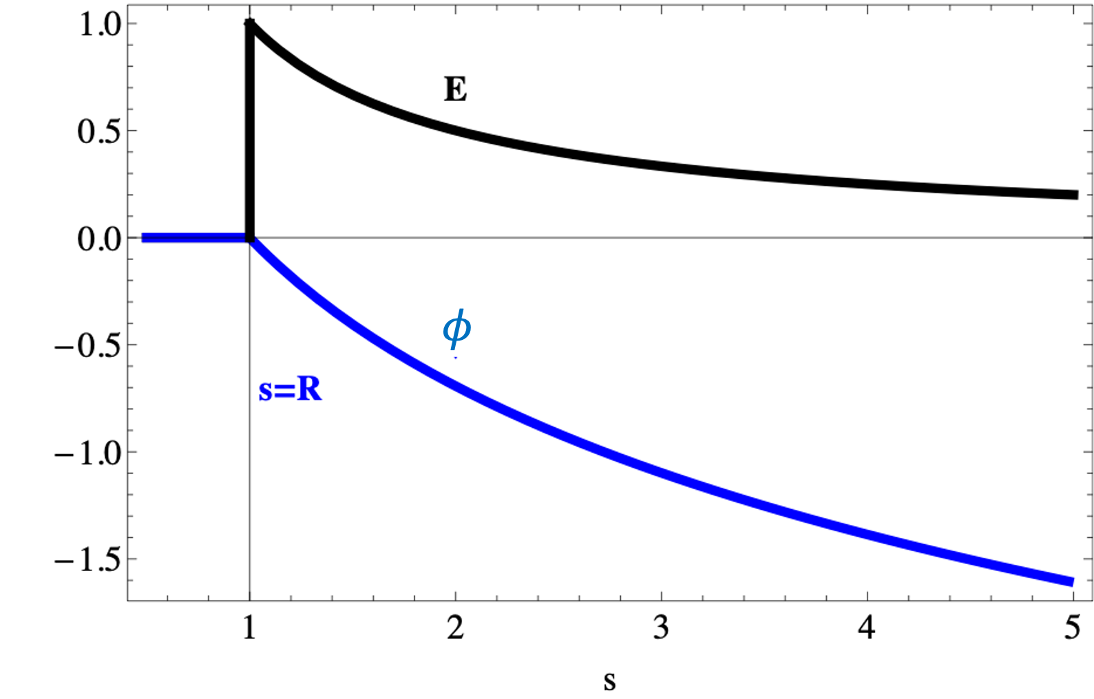
Since electric field goes to zero as \(1/r^2\) for large \(r\text{,}\) we can choose reference zero of potential at \(r=\infty\) and compute the following integral for an arbitrary point \(r_\text{P}\text{.}\)

\begin{equation*} V_\text{P} = -\int_\infty^{r_\text{P}}\, E(r)\, dr. \end{equation*}

For point P outside of all spheres, you will get

\begin{equation*} V_\text{P} = \frac{1}{4\pi\epsilon_0}\:\frac{-3\:\mu\text{C}}{r_\text{P}}. \end{equation*}

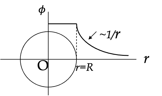
This is as if the net charge was placed at the center. For P between the shells, you will get (expressing the radius in units of meter.)

\begin{equation*} V_\text{P} = \frac{1}{4\pi\epsilon_0}\:\frac{-3\:\mu\text{C}}{0.08\text{ m}}. \end{equation*}

For P between the inner sphere and inner shell

\begin{equation*} V_\text{P} =\frac{1}{4\pi\epsilon_0}\:\left( \frac{-3\:\mu\text{C}}{0.08\text{ m}} + \frac{5\:\mu\text{C}}{r_\text{P}} - \frac{5\:\mu\text{C}}{0.06\,\text{ m}} \right) \end{equation*}

Finally, for point P inside the inner-most sphere

\begin{equation*} V_\text{P} = \frac{1}{4\pi\epsilon_0}\:\left( \frac{-3\:\mu\text{C}}{0.08\text{ m}} + \frac{5\:\mu\text{C}}{0.04\,\text{m}} - \frac{5\:\mu\text{C}}{0.06\,\text{ m}} \right) \end{equation*}

2. Electric Field of Charged Copper Cylinder.

A long cylinder of copper of radius \(3\text{ cm}\) is charged so that it has a uniform charge per unit length on its surface of \(3\;\mu\text{C/m}\text{.}\) (a) Find the electric field inside (\(s=2.0\text{ cm}\)) and outside (\(s=4.0\text{ cm}\)) the cylinder. (b) Draw electric field lines in a plane perpendicular to the rod. (c) Find electric potential at an arbitrary point using \(s=1.0\text{ cm}\) as the point for the zero potential reference even though this point is within the cylinder.

Hint.

(a) Use formula for electric field for cylindrical symmetry. (b) Use the rule that: (1) Electric field lines begin at positive charge and end at negative charges and (2) Electric field lines land perpendicularly on metals. (c) Do the integral of electric field.

Answer.

(a) \(1.35\times 10^6 \:\text{N/C}\text{,}\)(b) see solution. (c) left as an exercise.

Solution 1. (a)

(a) Since, we have electrostatic situation, charges on metal will reside on the surface of the cylinder. Using the Gauss’s law for cylindrical symmetry, you find that electric field inside the cylinder is zero.

\begin{equation*} E_\text{in} = 0. \end{equation*}

From using Gauss’s law for a point outside we will get

\begin{equation*} E_\text{out} = \frac{\lambda}{2\pi\epsilon_0}\;\frac{1}{s}, \end{equation*}

where \(s\) is the distance of the point from the center of the rod. at points outside the cylinder, the magnitude \(E_{\text{out}}\) of electric field is dependent on the distance \(s\) meters from the axis of the cylinder.

\begin{align*} E_{\text{out}} \amp = \frac{1}{2\pi\epsilon_0}\:\frac{\lambda}{s} = 2k\:\frac{\lambda}{s} \\ \amp = 2\times 9\times 10^{9}\:\frac{\text{N.m}^2}{\text{C}^2}\times \frac{3\times 10^{-6}\:\text{C/m}}{0.04\:\text{m}} = 1.35\times 10^6 \:\text{N/C}. \end{align*}

Solution 2. (b)

Figure 32.28 shows electric field lines and equi-potential lines (dashed) in a cross-section of the wire.

3. Electric Potential between two Charged Metal Plates.

Two large charged aluminum plates of charge density \(\pm 30\text{ mC/m}^2\) face each other at a separation of \(5\text{ mm}\text{.}\) (a) Find the electric potential everywhere. (b) An electron is released from rest at the negative plate, with what speed will it strike the positive plate?

Hint.

(a) Electric field between plates is constant. (b) Use conservation of energy.

Answer.

(a) \(1.69\times 10^7\:\text{V}\text{,}\) (b) \(5.7\times 10^7\text{ m/s}\text{.}\)

Solution 1. (a)

(a) The electric field between the plates is constant with magnitude \(E = \sigma/\epsilon_0\) directed from the positive plate to the negative plate. Therefore the electric potential between the plates increases linearly from zero on the negative plate to \(\phi = (\sigma/\epsilon_0)\:d\) on the positive plate, where \(d\) is the separation of plates. The numerical value of the potential difference will be

\begin{equation*} \phi = \frac{30\times 10^{-3}\:\text{C/m}^2}{8.85\times 10^{-12}\:\text{C}^2/\text{N.m}^2}\:0.005\:\text{m} = 1.69\times 10^7\:\text{V}, \end{equation*}

where I have written the final unit as volts since that is what the combination of the other units is called in SI units.

Solution 2. (b)

(b) Using the conservation of energy we find

\begin{equation*} \frac{1}{2} mv^2 = |e\: \phi| \end{equation*}

Hence,

\begin{align*} v \amp = \sqrt{2|e\: \phi|/m}\\ \amp = \sqrt{2\times 1.6\times 10^{-19}\:\text{C}\times 1.69\times 10^7\:\text{V}/1.67\times 10^{-27}\:\text{kg}}\\ \amp = 5.7\times 10^7\:\text{m/s}, \end{align*}

which is about 1/5th of the speed of light in vacuum. You should probably use relativistic formulas.

4. Charge and Voltage of a Gold Shell Surrounding a Charged Pith Ball.

A small spherical pith ball of radius \(0.5\text{ cm}\) is painted with a silver paint and then \(-10\ \text{nC}\) of charge placed on it. The charged pith ball is put at the center of a gold spherical shell of inner radius \(2.0\text{ cm}\) and outer radius \(2.2\text{ cm}\text{.}\)

(a) Find the electric potential of the gold shell with respect to zero potential at infinity.

(b) How much charge should you put on the gold shell if you want to make its potential \(100\text{ V}\text{?}\)

Hint.

(a) Outside the spherical gold shell, formula for potential is same as that of a point charge located at the origin. (b) Set up the condition for potential at outer surface of gold shell.

Answer.

(a) \(4.1\text{ kV}\text{,}\) (b) \(10.244\text{ nC}\text{.}\)

Solution 1. (a)

(a) Outside the gold shell, the potential will be given by the same formula as that of a point charge at the center. Therefore,

\begin{align*} \phi \amp = \frac{1}{4\pi\epsilon_0}\: \frac{q}{R}\\ \amp = 9\times 10^9\:\text{N.m}^2\text{/C}^2\times\frac{-10\times 10^{-9}\:\text{C}}{0.022\:\text{m}} = - 4.1\times 10^{3}\;\text{V}. \end{align*}

Solution 2. (b)

(b) To make the potential of the gold shell \(100\text{ V}\text{,}\) we must put positive charge \(Q\) on the shell such that its potential and that of the charges on the pith ball together equal \(100\text{ V}\text{.}\) This gives the following condition on \(Q\text{.}\)

\begin{equation*} 9\times 10^{9}\:\text{N.m}^2\text{/C}^2\times\frac{-10\times 10^{-9}\:\text{C} + Q}{0.022\:\text{m}} = 100\:\text{V}. \end{equation*}

When you solve this equation for \(Q\) you get

\begin{equation*} Q = \left[ 10\times 10^{-9} + 2.44\times 10^{-10} \right]\: \text{C} = 10.244\text{ nC}. \end{equation*}

5. Electric Field and Electric Potential of a Charged Aluminum Cylinder.

A long cylinder of aluminum of radius \(R\) is charged so that it has a uniform charge per unit length on its surface of \(\lambda\text{.}\) (a) Find the electric field inside and outside the cylinder. (b) Find the electric potential inside and outside the cylinder. (c) Plot electric field and electric potential as a function of distance from the center of the rod.

Hint.

Use Gauss’s law.

Answer.

(a) \(E_{\textrm{in}} = 0\text{,}\) \(E_{\textrm{out}} = \frac{\lambda}{2\pi\epsilon_0}\: \frac{1}{s}\text{,}\) (b) \(\phi_{\textrm{in}} = 0\text{,}\) \(\phi_{\textrm{out}} = -\frac{\lambda}{2\pi\epsilon_0}\: \ln\frac{s}{R}\text{,}\) (c) See solution.

Solution 1. (a)

(a) By Gauss’s law, you can show that \(E_{\textrm{in}} = 0\text{,}\) and \(E_{\textrm{out}}\) is given by the following.

\begin{equation*} E_{\textrm{out}} = \frac{\lambda}{2\pi\epsilon_0}\: \frac{1}{s},\ \ \ (s>R) \end{equation*}

The direction of the elctric field is (cylindrical) radially out from the axis of the cylinder if \(\lambda \gt 0\) and towards the axis if \(\lambda \lt 0\text{.}\)

Solution 2. (b)

(b) The electric potential at a field point can be obtained by integrating electric field from a reference point a distance \(s_{\textrm{ref}}\) from the axis to the field point. For simplicity we can pick \(s_{\textrm{ref}} = R\) so that potential at the surface of the cylinder will be zero. In this case we get integrating the electric field from \(s=R\) to \(s \gt R\text{,}\) we get

\begin{equation*} \phi_{\textrm{out}} = -\frac{\lambda}{2\pi\epsilon_0}\: \ln\frac{s}{R}\ \ (s\ge R). \end{equation*}

The electric potential inside does not change from that at the outer surface of the metal since electric field in the body of the aluminum cylinder is zero. Hence,

\begin{equation*} \phi_{\textrm{in}} = 0\ \ (s\le R). \end{equation*}

Solution 3. (c)

(c) The plot for electric field and electric potentials are shown in the figure below. Note that while the magnitude of the electric field has a jump across the metal, the electric potential is continuous.

Prev Top Next