   
Logo image

Physics Bootcamp

Section 9.4 Rotational Acceleration

Just as angular velocity \(\omega \) is the rate of change of rotation angle \(\theta\text{,}\) angular acceleration is the rate of change of angular velocity \(\omega\text{.}\) Angular acceleration is also called rotational acceleration. We denote angular acceleration by the Greek letter \(\alpha\) (alpha).
Similar to the average angular velocity, we have average angular acceleration. This refers to net angular acceleration averaged over some period of time. An instantaneous angular acceleration refers to the angular acceleration at a particular instant.
It is important to note that angular acceleration is a vector quantity. In the following we will be working in a fixed-axis rotation and use simple notation of using only velocity and acceleration components along the axis of rotation, which will be taken to define the \(z\)-axis of the reference frame.

Subsection 9.4.1 Average Angular Acceleration

By dividing the change in (instantaneous) angular velocity by the time interval we get the average angular acceleration for that time interval. Consider an interval from \(t_i \) to \(t_f\text{.}\) Let the instantaneous angular velocity at these instants be \(\omega_i \hat k\) and \(\omega_f \hat k\text{,}\) where we are including the axis of rotation information. Then, the average angular acceleration, \(\vec \alpha_{\text{av}}\) will be
\begin{equation} \vec \alpha_{\text{av}} = \left( \dfrac{\omega_f - \omega_i }{t_f - t_i} \right)\, \hat k \equiv \dfrac{\Delta \omega }{\Delta t}\, \hat k.\tag{9.9} \end{equation}
Since we will be working exclusively with axis of rotation along the \(z\)-axis, it is not a problem to work with just the component part and drop off the \(\hat k\) from our formulas. This should not cause any problem.
\begin{equation} \alpha_{\text{av}} = \dfrac{\omega_f - \omega_i }{t_f - t_i} \equiv \dfrac{\Delta \omega }{\Delta t}.\tag{9.10} \end{equation}

Subsection 9.4.2 Instantaneous Angular Acceleration

Often we want angular acceleration at a particular instant. What we mean by this is the average angular acceleration between that instant, say \(t \) and an instant very close to \(t\text{,}\) say, \(t + \Delta t \) where \(\Delta t\) is an infinitesimal time.
Denoting the instantaneous angular acceleration by symbol \(\alpha \text{,}\) we write this special average quantity formally as
\begin{equation} \alpha = \dfrac{\omega\left(\text{at } (t+\Delta t)\right) - \omega\left(\text{at } t\right)}{\Delta t} = \frac{\Delta \omega}{\Delta t}.\tag{9.11} \end{equation}
Here, it is understood that a limit \(\Delta t \rightarrow 0\) is to be taken in these expressions. With the limit included, we also write it as a derivative.
\begin{equation} \alpha = \frac{d\omega}{dt}.\tag{9.12} \end{equation}
Since \(\alpha \) is a ratio of a change in \(\omega \) to a change in \(t \) it can be computed by the slope of \(\omega \) versus \(t\) plot.
The angular acceleration is a vector quantity. Therefore, it has a direction and a magnitude. The direction for a fixed-axis rotation wil either be in the direction of the axis of rotation or in the opposite direction as illustrated in Figure 9.24.
Figure 9.24.
To tell the direction of angular acceleration, you will need to look at the direction of angular velocity and whether the motion is slowing or speeding up. The angular velocity is in the direction of the axis if the object is rotating counterclockwise otherwise it is in the opposite direction. The angular acceleration will then be in the direction of the angular velocity or opposite to it depending upon whether the rotation is speeding up or slowing down.

Example 9.25. Signs of Angular Velocity and Angular Acceleration.

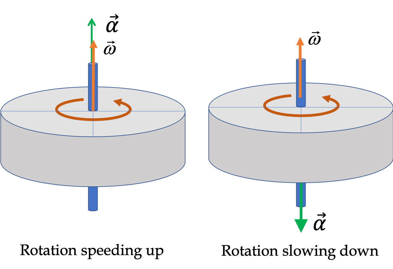
For instance, if angular velocity is 30 rad/sec counterclockwise and the rotation is slowig down at a rate of 5 rad/sec per second. Then, \(\omega = 30\text{ rad/sec}\) and \(\alpha = -5 \text{ rad/sec}^2\text{.}\) If the rotation was speeding up, \(\alpha = +5 \text{ rad/sec}^2\text{.}\)
On the other hand if angular velocity is 30 rad/sec clockwise and the rotation is slowig down at a rate of 5 rad/sec per second. Then, \(\omega = -30\text{ rad/sec}\) and \(\alpha = +5 \text{ rad/sec}^2\text{,}\) and if speeding up, \(\alpha = -5 \text{ rad/sec}^2\text{.}\) Speeding up means acceleration has same direction as velocity and slowing down means they are in the opposite direction.

Subsection 9.4.3 Instantaneous Angular Acceleration - Graphically

The rate of change of \(\omega \) at an instant can be computed by the slope of the tangent to \(\omega \) versus \(t \) plot - similar to the way we defined the rate of chang of \(x \text{.}\)
If angular velocity is increasing or decreasing at a constant rate, we say the object has uniform angular acceleration. An example is shown in Figure 9.26.
Since \(\omega \) versus \(t \) plot is a straight line, angular velocity changes uniformly wth time with a constant acceleration. From slope, we get angular acceleration, \(\alpha\text{.}\)
\begin{equation*} \alpha = \alpha_\text{av} = \dfrac{\omega_2 - \omega_1}{t_2 - t_1}. \end{equation*}
Figure 9.26.
On the other hand, if the angular velocity is increasing or decreasing at a non-constant rate, \(\omega \) versus \(t \) plot will not be a straight line. An example is shown in Figure 9.27. In this case, slope of tangent to the curve at the instant of interest gives acceleration at that instant.
The figure shows tangent lines for instants \(t_1 \) and \(t_2\text{.}\) The slope of the tangent lines \(L_1 \) and \(L_2\) are then the instantaneous angular accelerations at these instants.
Figure 9.27.

Example 9.28. Angular Acceleration from Angular Velocity versus Time Plot - Linear Segments.

Figure 9.29 shows the angular velocity of a rotating fan at different times. We wish to study this plot and determine the following aspects of the rotation.
(a) Is the rotation at (i) \(t = 5\text{ sec} \text{,}\) (ii) \(t = 15\text{ sec} \text{,}\) (iii) \(t = 25\text{ sec} \text{,}\) (iv) \(t = 35\text{ sec} \text{,}\) (v) \(t = 45\text{ sec} \text{,}\) (vi) \(t = 55\text{ sec} \text{,}\) clockwise or a counterclockwise or no rotation? How can you tell?
(b) What are the values of instantaneous angular accelerations at (i) \(t = 5\text{ sec} \text{,}\) (ii) \(t = 15\text{ sec} \text{,}\) (iii) \(t = 25\text{ sec} \text{,}\) (iv) \(t = 35\text{ sec} \text{,}\) (v) \(t = 45\text{ sec} \text{,}\) (vi) \(t = 55\text{ sec} \text{?}\)
(c) What are the average accelerations during the following intervals (i) \(t = 0 \) to \(t = 20\text{ sec} \text{,}\) (ii) \(t = 20\text{ sec} \) to \(t = 30\text{ sec} \text{,}\) (iii) \(t = 30\text{ sec} \) to \(t = 40\text{ sec} \text{,}\) (iv) \(t = 40\text{ sec} \) to \(t = 50\text{ sec} \text{,}\) (v) \(t = 50\text{ sec} \) to \(t = 60\text{ sec} \text{,}\) and (vi) \(t = 0 \) to \(t = 60\text{ sec} \text{.}\)
Figure 9.29. Figure for Example 9.28.
Answer.
(a) Counterclockwise: (i), (ii), (iii); No rotation at (iv), and clockwise at (v), and (vi). (b) (i) \(1\text{ rad/sec}^2\text{,}\) (ii) \(1\text{ rad/sec}^2\text{,}\) (iii) \(0\text{,}\) (iv) \(-4\text{ rad/sec}^2\) , (v) \(1\text{ rad/sec}^2\) , and (vi) \(0\text{.}\) (c) (i) \(1\text{ rad/sec}^2\text{,}\) (ii)\(0\text{,}\) (iii) \(-4\text{ rad/sec}^2\) , (iv) \(1\text{ rad/sec}^2\) , (v) \(0\text{,}\) and (vi) \(-\dfrac{1}{6}\,\text{ rad/sec}^2\text{.}\)
Solution 1. a
From the definition of angular velocity, we know that a clockwise rotation will have a negative value of \(\omega \) and a counterclockwise rotation a positive value. Therefore, we can answer this question immediately from reading off the sign of \(\omega \text{.}\)
Counterclockwise at (i) \(t = 5\text{ sec} \text{,}\) (ii) \(t = 15\text{ sec} \text{,}\) and (iii) \(t = 25\text{ sec} \text{,}\)
no rotation at (iv) \(t = 35\text{ sec} \text{,}\) and
Clockwise at (v) \(t = 45\text{ sec} \text{,}\) and (vi) \(t = 55\text{ sec} \text{.}\)
Solution 2. b
Since the segments are all linear, we do not need to draw any tangents; we just use the slope of the line upon which the point of interest falls.
(i) The slope here is
\begin{equation*} \alpha = \dfrac{20-0}{20-0} = 1\text{ rad/sec}^2. \end{equation*}
(ii) We do not need to do any work. This is same as (i).
(iii) The angular velocity is not changing here. Therefore, the slope here is zero. Hence, \(\alpha = 0\text{.}\)
(iv) the slope here is
\begin{equation*} \alpha = \dfrac{-20-20}{40-30} = -4\text{ rad/sec}^2. \end{equation*}
(v) The slope here is
\begin{equation*} \alpha = \dfrac{-10-(-20)}{50-40} = 1\text{ rad/sec}^2. \end{equation*}
You could have just used the parallel nature of this line to the line for (i) and guessed the answer.
(vi) The angular velocity is not changing here. Hence, \(\alpha = 0\text{.}\)
Solution 3. c
We just use the values of angular velocity and times at the end points of the segment and calculate the slopes. The slopes here will give us the average angular accelerations, and not the instantaneous angular accelerations.
(i) The slope here is
\begin{equation*} \alpha_{\text{av}} = \dfrac{20-0}{20-0} = 1\text{ rad/sec}^2. \end{equation*}
(ii) The angular velocity at the two ends is same. Therefore, the slope here is zero. Hence, \(\alpha_{\text{av}} = 0\text{.}\)
(iii) the slope here is
\begin{equation*} \alpha_{\text{av}} = \dfrac{-20-20}{40-30} = -4\text{ rad/sec}^2. \end{equation*}
(iv) The slope here is
\begin{equation*} \alpha_{\text{av}} = \dfrac{-10-(-20)}{50-40} = 1\text{ rad/sec}^2. \end{equation*}
(v) The final angular velocity is same as initial angular velocity, here. Hence, \(\alpha_{\text{av}} = 0\text{.}\)
(vi) The slope here is
\begin{equation*} \alpha_{\text{av}} = \dfrac{-10-0}{60-0} = -\dfrac{1}{6}\,\text{ rad/sec}^2. \end{equation*}