Logo image

Physics Bootcamp

Section 2.5 Acceleration

Acceleration is an important characteristic of motion. It connects the motion of an object to the influence of environment on the motion. In this first exposure to this topic, we will focus on motion along \(x\)-axis only. In a later chapter we will study acceleration in a more general setting.
Similar to our treatment of velocity, we will define an average acceleration and an instantaneous acceleration. For a motion on the \(x \) axis, we will denote instantaneous acceleration by symbol \(a_x\) and average acceleration by \(a_{\text{av},x}\text{.}\)

Subsection 2.5.1 Average Acceleration

The average rate of change of velocity during a finite interval can be obtained by dividing the change in velocity by the interval. Let \(v_{i,x} \) be the (instantaneous) velocity at instant \(t_i\) and \(v_{f,x} \) be the (instantaneous) velocity at instant \(t_f\text{,}\) then average acceleration, \(a_{\text{av},x}\) during \(t_i\) to \(t_f\text{,}\) will be
\begin{equation} a_{\text{av},x} = \dfrac{v_{f,x} - v_{i,x}}{ t_f - t_i}.\tag{2.9} \end{equation}
You can see that writing all the subscripts can be too tedious. So, if there is no confusion that we are working along one axis and that we are dealing with average acceleration, we can write this definition much more simply by dropping off all the unnecessary subscripts as follows.
\begin{equation*} a = \dfrac{v_{f} - v_{i}}{ t_f - t_i}. \end{equation*}
However, for the sake of being specific and completeness, in the book I will continue to add all the necessary subscripts, but in your studies, you don’t have to bother as long as you are clear about what you are suppressing. By writing \(\Delta v_x\) for \(v_{f,x} - v_{i,x}\) and \(\Delta t\) for \(t_f - t_i\text{,}\) we often write this as
\begin{equation*} a_{\text{av},x} = \dfrac{\Delta v_x}{ \Delta t}, \end{equation*}
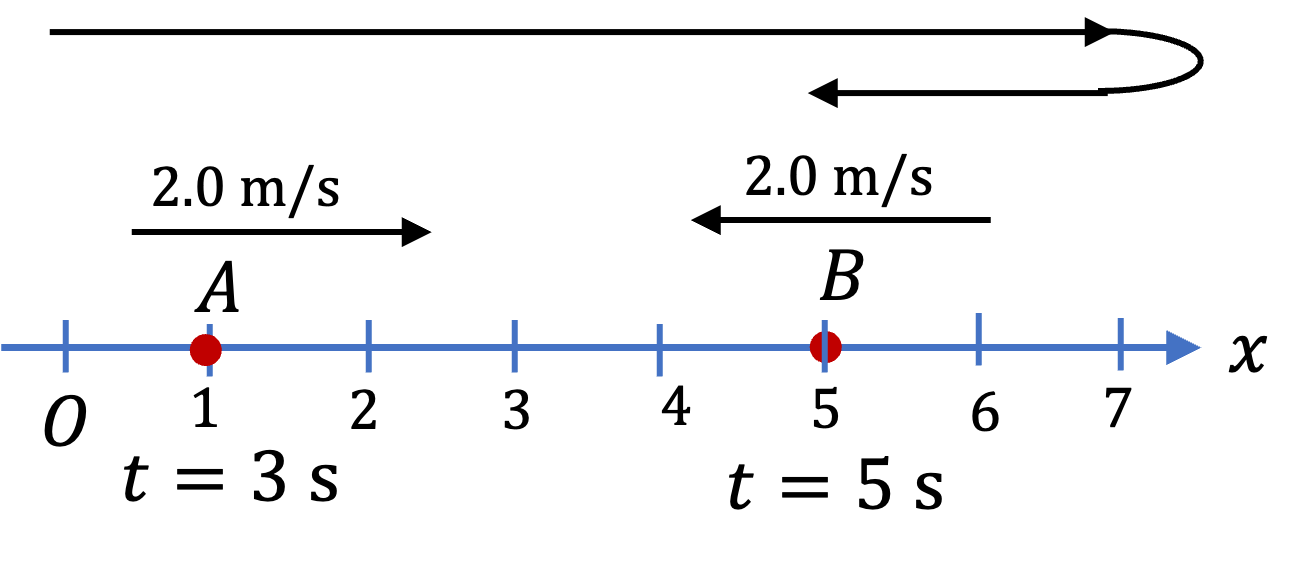
Note that for average aceleration, we do not need to know the details of the motion at any instant other than what happened at just the initial and final instants. For instance, for a motion shown in Figure 2.39, the average acceleration between A and B will be obtained from \(v_x\) at those points and time between them.
Note that \(v_x(\text{at B})\) is negative since the particle is moving towards negative \(x\) axis although it is on the positive \(x\)-axis.
\begin{align*} \amp v_x(A) = 2.0\text{ m/s}, \\ \amp v_x(B) = - 2.0\text{ m/s}, \\ \amp a_{\text{av},x} = \frac{-2.0-2.0}{2.0} = -2.0\text{ m/s}^2. \end{align*}
Figure 2.39.

Example 2.40. Change in Velocity from Average Acceleration.

A box is moving on \(x\)-axis with velocity of \(+12.0\text{ m/s}\) and has a constant acceleration of \(-9.0\text{ m/s}^2\text{.}\) Find its velocity after (a) 1\text{ sec}, (b) 2\text{ s}.
Answer.
(a) \(+3.0\text{ m/s}\text{,}\) (b) \(-6.0\text{ m/s}\text{.}\)
Solution 1. a
If the acceleration is constant, then this acceleration is same as average acceleration. From the definition of average acceleration we have the change in velocity to be
\begin{equation*} \Delta v_x = a_x\, \Delta t. \end{equation*}
Therefore in one second
\begin{equation*} \Delta v_x = -9.0 \times 1 = -9.0\text{ m/s}. \end{equation*}
Adding this to the initial velocity gives
\begin{equation*} v_x(\text{at }t=1\text{ sec}) = v_{ix} + \Delta v_x = 12 - 9 = 3.0\text{ m/s}. \end{equation*}
Solution 2. b
In 2 sec:
\begin{equation*} \Delta v_x = -9.0 \times 2 = -18.0\text{ m/s}. \end{equation*}
Adding this to the initial velocity gives
\begin{equation*} v_x(\text{at }t=2\text{ sec}) = v_{ix} + \Delta v_x = 12 - 18 = -6.0\text{ m/s}. \end{equation*}
The negative sign here means the object is not moving in the direction of the negative \(x\)-axis.

Subsection 2.5.2 Instantaneous Acceleration

Often we want acceleration at a particular instant, called instantaneous acceleration, or simply, acceleration. This is the rate of change of velocity at that instant. Again, here we just look at a one-dimensional motion on the \(x\)-axis and defer the more complete treatment to a later chapter.
Consider an arbitrary motion on \(x\)-axis. Let \(v_x\left(\text{at } t\right)\) be the \(x\)-velocity at instant \(t\) and \(v_x\left(\text{at } t+\Delta t\right)\) at instant \((t+\Delta t)\text{.}\) Then, \(x\)-acceleration \(a_x\) AT INSTANT \(t\) will be defined by the limiting process of taking the duration \(\Delta t\) as close to zero as possible except \(\Delta t = 0\text{.}\)
\begin{equation} a_x = \lim_{\Delta t \rightarrow 0}\dfrac{v_x\left(\text{at } t+\Delta t\right) - v_x\left(\text{at } t\right)}{\Delta t}.\tag{2.10} \end{equation}
Of course, we also denote this process by a simler notation of the derivative symbol, \(dv_x/dt\text{,}\) where we think of \(v_x\) as a continuous function of \(t\text{.}\)
\begin{equation} a_x = \dfrac{dv_x}{dt}.\tag{2.11} \end{equation}
Recall that graphically, the derivative of a function is also slope of tangent at that point. Here, we look at the plot of \(v_x\) (on the ordinate) versus \(t\) (on the abscissa). Then, \(a_x\) can be computed by the slope of the tangent to the \(v_x \) versus \(t\) at the instant of interest.

Remark 2.41. Positive and Negative \(a_x\) do not tell direction of motion.

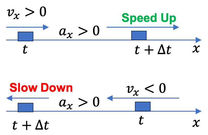
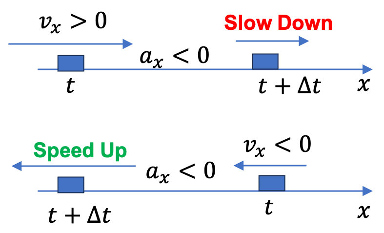
Recall that positive \(v_x\) corresponded to the object moving towards \(x=+\infty\) and negative \(v_x\) corresponded to moving towards \(-\infty\text{.}\) But, positive and negative \(a_x\) do not have such simple interpretations. Positive \(a_x\) means the \(v_x\) of the motion is becoming more positive with time and negative \(a_x\) means \(v_x\) of the motion is becoming more negative with time. Let us look at two important cases.

Example 2.42. Positive \(a_x\).

Positive \(a_x\) adds positive velocity values to \(v_x\text{.}\) Thus if an object is initially moving towards positive \(x\)-axis, it will speed up and if it was moving towards the negative \(x\)-axis, it will slow down. In this later case, if \(a_x\) remains the same, the object will eventually turn around and move towards positive \(x\)-axis, i.e., \(v_x\) eventually becoming positive.

Example 2.43. Negative \(a_x\).

Negative \(a_x\) adds negative velocity values to \(v_x\text{.}\) Thus if an object is initially moving towards negative \(x\)-axis, it will speed up and if it was moving towards the positive \(x\)-axis, it will slow down. In this later case, if \(a_x\) remains the same, the object will eventually turn around and move towards negative \(x\)-axis, i.e., \(v_x\) eventually becoming negative.

Example 2.44. (Calculus) Velocity and Acceleration from Derivative.

In theoretical work you might find that you are given position as a function \(x(t) \text{.}\) For example, a block attached to a spring oscillates with its position \(x(t) = (5 \text{ cm}) \cos( 2\pi t)\text{,}\) where \(t \) is in seconds. If you plot this \(x \) versus \(t \text{,}\) you will notice that the block moves between \(x = - 5 \) cm and \(x = 5 \) cm, repeating a complete cycle every second.
(a) What is the velocity of this block at (i) \(t = 0.25 \) s, (ii) \(t = 0.5 \) s, and (iii) \(t = 0.75 \) s.
(b) What is the acceleration of this block at (a) \(t = 0.25 \) s, (b) \(t = 0.5 \) s, and (c) \(t = 0.75 \) s.
Answer.
(a) (i) \(-10\pi\text{ cm/s}\text{,}\) (ii) \(0\text{,}\) (iii) \(10\pi\text{ cm/s}\text{,}\) (b) (i) \(0\text{,}\) (ii) \(20\pi^2 \text{ cm/s}^2\text{,}\) (iii) \(0\text{.}\)
Solution 1. a
Taking the derivative of given \(x(t) \) and then evaluating the result at the required times should give us the answers.
\begin{equation*} v_x = \dfrac{dx}{dt} = (-10\pi \text{ cm/s}) \sin(2\pi t). \end{equation*}
(i) \(v_x = (-10\pi \text{ cm/s}) \sin(2\pi \times 0.25) = -10\pi \text{ cm/s} = -31.4 \text{ cm/s}. \)
(ii) \(v_x = (-10\pi \text{ cm/s}) \sin(2\pi \times 0.50) = 0. \)
(iii) \(v_x = (-10\pi \text{ cm/s}) \sin(2\pi \times 0.75) = 10\pi \text{ cm/s}= 31.4 \text{ cm/s}. \)
Solution 2. b
Taking the derivative of \(v_x \) and then evaluating the result at the requires times should give us the answers.
\begin{equation*} a_x = \dfrac{dv_x}{dt} = (-20\pi^2 \text{ cm/s}^2) \cos(2\pi t). \end{equation*}
(i) \(a_x = (-20\pi^2 \text{ cm/s}^2) \cos(2\pi \times 0.25) = 0. \)
(ii) \(a_x = (-20\pi^2 \text{ cm/s}^2) \cos(2\pi \times 0.50) = 20\pi^2 \text{ cm/s}^2. \)
(iii) \(a_x = (-20\pi^2 \text{ cm/s}^2) \cos(2\pi \times 0.75) = 0. \)

Subsection 2.5.3 Graphical Definition of Acceleration

Since the slope of a function is the rate of change of that function, the rate of change of velocity at a particular instant can be obtained from the slope of the tangent of the velocity versus time plot. We can take this as defining acceleration \(a_x \) for one-dimensional motion on the \(x \) axis.
\begin{equation} a_x = \text{ slope of tangent to }v_x\text{ versus }t.\tag{2.12} \end{equation}
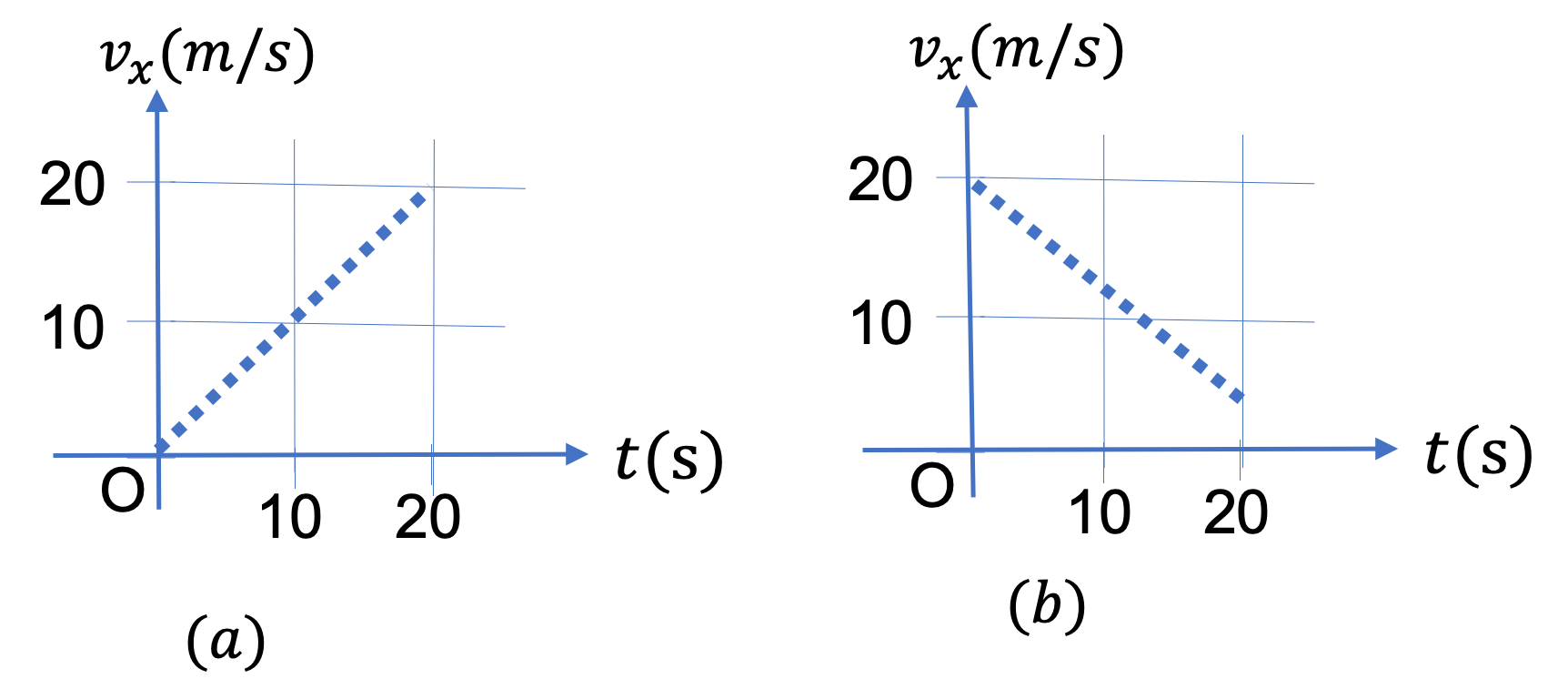
If the plot of \(v_x \) versus \(t \) is linear, i.e., a straight line as in Fig. Figure 2.45, then the tangent line is same as the line of the plot, hence \(a_x \) is just the slope of the line.
Figure 2.45. The slope of \(v_x \) versus \(t \) plot gives the acceleration \(a_x \text{.}\) Since the plot is linear, the slope is same for all instants plotted. In (a) \(a_x = 1.0 \text{ m/s}^2\) and in (b) \(a_x = - 0.75 \text{ m/s}^2\text{.}\)
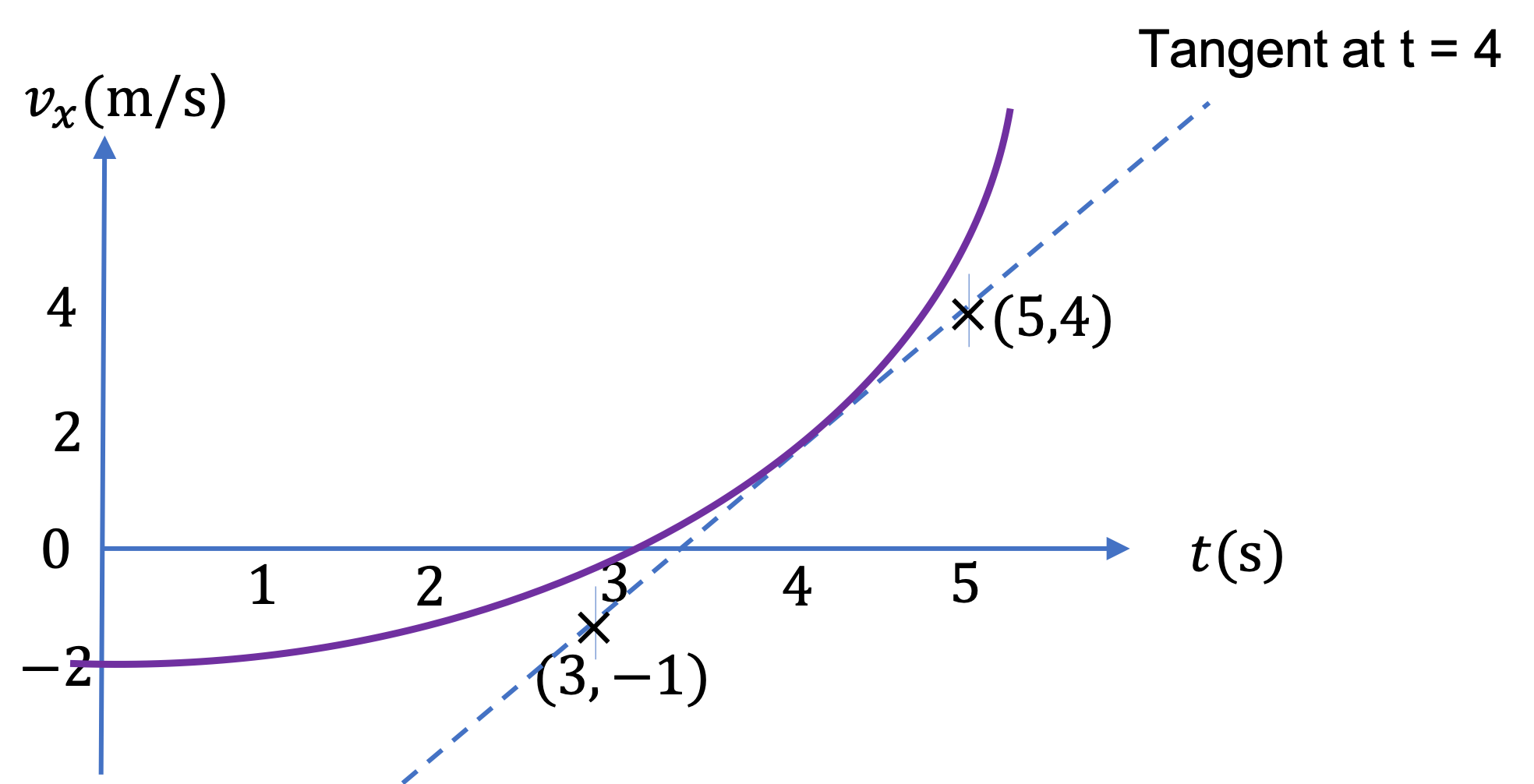
But, if the plot of \(v_x \) versus \(t \) is curved as in Figure 2.46, then you would draw a tangent line at the instant of interest, and compute the slope of the tangent line to get \(a_x \text{.}\)
Figure 2.46. The slope of \(v_x \) versus \(t \) plot gives the acceleration \(a_x \text{.}\) Since the plot is not linear, we need to first draw a tangent line at the instant we want the acceleration value. The figure illustrates \(a_x\) at \(t = 4\text{ sec}\text{,}\) where the slope of the tangent line is \(a_x = (4-(-1))/(5-3) = 2.5\text{ m/s}^2 \text{.}\)

Example 2.47. Using slope of \(v_x \) to compute \(a_x \).

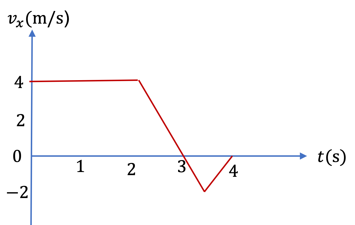
From the \(v_x \) versus \(t \) plot in Figure 2.48, find \(a_x \) at the following instants: (a) \(t = 1\text{ sec}\text{,}\) (b) \(t = 3\text{ sec} \text{,}\) and (c) \(t = 3.75\text{ sec} \text{.}\)
Figure 2.48. Figure for Example 2.47.
Answer.
(a) \(0\text{,}\) (b) \(-4\text{ m/s}^2\text{,}\) (c) \(4\text{ m/s}^2\)
Solution 1. a
(a) The \(v_x \) versus \(t\) plot through the time when \(t = 1\text{ sec}\) is a straight line. Therefore, \(a_x \) will simply be slope of this part of the plot. The slope of this line is clearly zero. Therefore, \(a_x (\text{at }t=1\text{ sec}) = 0\text{.}\)
(b) The \(v_x \) versus \(t\) plot through the time when \(t = 3\text{ sec}\) is a straight line. Therefore, \(a_x \) will simply be slope of this part of the plot. The slope of this line is obtained by picking two points on the line between \(t = 2\text{ sec}\) and \(t = 3.5\text{ sec}\text{.}\) We pick points at \(t = 2\text{ sec}\) and \(t = 3\text{ sec}\) to obtain
\begin{equation*} a_x = \dfrac{0 - 4\text{ m/s}}{3\text{ s}-2\text{ s}} = -4\text{ m/s}^2. \end{equation*}
Solution 2. b
The \(v_x \) versus \(t\) plot through the time when \(t = 3.75\text{ sec}\) is a straight line. Therefore, \(a_x \) will simply be slope of this part of the plot. The slope of this line is obtained by picking two points on the line between \(t = 3.5\text{ sec}\) and \(t = 4.0\text{ sec}\text{.}\) We pick points at \(t = 3.5\text{ sec}\) and \(t = 4\text{ sec}\) to obtain
\begin{equation*} a_x = \dfrac{0 - (-2)\text{ m/s}}{4\text{ s}-3.5\text{ s}} = 4\text{ m/s}^2. \end{equation*}

Subsection 2.5.4 Change in Velocity from Acceleration

Suppose a motion is along \(x\)-axis with velocity \(v_x\) at instant \(t\) and \((v_x+\Delta v_x) \) at instant \(t + \Delta t\text{.}\) Here \(\Delta v_x\) stands for whatever is the change in velocity during the interval. Then, recall that average acceleration for the finite interval \(t\) to \(t + \Delta t\) will be
\begin{equation*} a_{x,av} = \frac{(v_x + \Delta v_x) - v_x}{ (t + \Delta t) - t} = \frac{\Delta v_x}{\Delta t}. \end{equation*}
Then, we can immediately get the change in velocity \(\Delta v_x\) by multiplying both sides by the interval \(\Delta t\text{.}\)
\begin{equation*} \Delta v_x = a_{x,av}\,\Delta t. \end{equation*}
How about getting the change in velocity \(\Delta v_x\) from instantaneous acceleration \(a_x\) given at each instant between \(t\) and \(t + \Delta t\text{?}\) Since \(a_x\) is the derivative of the instantaneous velocity taken as a function of time, \(v_x(t)\text{,}\) to get the change in \(v_x\text{,}\) we will need to integrate \(a_x\text{,}\) which is itself a function of \(t\text{.}\) Let us denote \(t_i\) for the intitial instant and \(t_f\) for the final instant, and \(v_{x,f}-v_{x,i}\) for \(\Delta v_x\text{.}\)
\begin{equation} a_x = \frac{dv_x}{dt}\ \ \longleftrightarrow\ \ v_{x,f} - v_{x,i} = \int_{t_i}^{t_f}\, a_x(t)\,dt.\tag{2.13} \end{equation}
Now, an integral has a nice graphical interpretation - it is the area "under or over" the curve! You have already seen this in the context of velocity/displacement relation.
\begin{equation*} v_x = \frac{dx}{dt}\ \ \longleftrightarrow\ \ x_f - x_i = \int_{t_i}^{t_f}\, v_x(t)\,dt. \end{equation*}
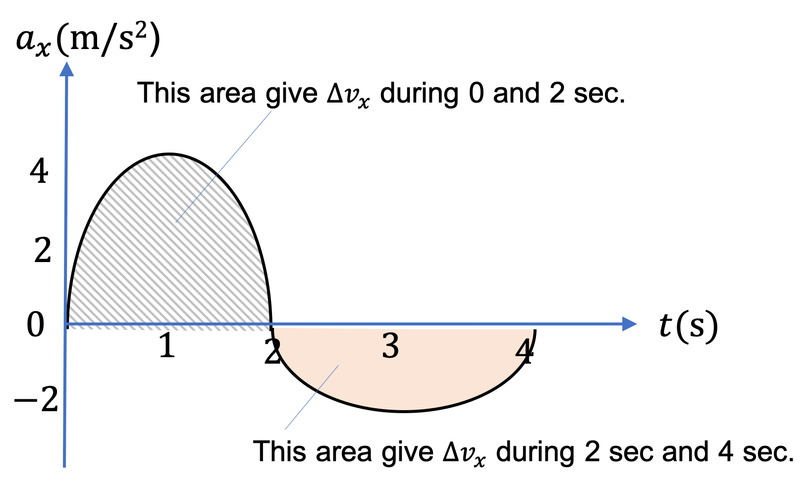
The corresponding ideas of area under the curve when the curve is above the abscissa and over the curve if below the abscissa is illustrated in Fig. Figure 2.49.
Figure 2.49. The area under the curve to get \(\Delta v_x \) from \(a_x\) versus \(t \) plot. The area for the curve when \(a_x \gt 0\) is positive, as between \(t=0 \) and \(t= 2\text{ sec}\) and the area for the curve when \(a_x \lt 0\) is negative, as between \(t= 2\text{ sec} \) and \(t= 4\text{ sec}\text{.}\)

Example 2.50. Compute \(\Delta v_x \) from \(a_x\) versus \(t \) plot.

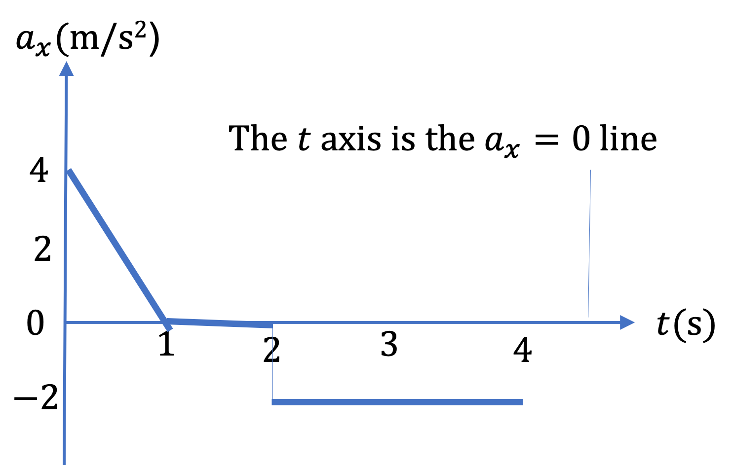
A ball is initially (\(t=0 \)) moving at \(v_x = 3\text{ m/s}\text{.}\) The acceleration of the ball at different times are as shown in the \(a_x \) versus \(t \) plot in Figure 2.51. Find \(v_x \) at (a) \(t = 1\text{ sec} \text{,}\) (b) \(t = 2\text{ sec} \text{,}\) and (c) \(t = 4\text{ sec} \text{.}\)
Figure 2.51. Figure for Example 2.50.
Answer.
(a) \(5\text{ m/s}\text{,}\) (b) \(5\text{ m/s}\) , (c) \(1\text{ m/s} \text{.}\)
Solution 1. a
From the area-under-curve we can find the change in \(v_x \) during \(t= 0 \) to \(t = 1\text{ sec}\text{.}\) Adding this change to the \(v_x \) at \(t= 0\) will give us the \(v_x \) at \(t=1\text{ sec}\text{.}\)
\begin{equation*} \Delta v_x = \dfrac{1}{2}\times 4 \times 1 = 2\text{ m/s}. \end{equation*}
Therefore, \(v_x \) at \(t=1\text{ sec}\text{:}\)
\begin{equation*} v_x(\text{ at }t=1\text{ sec }) = v_x(\text{ at }t=0\ ) + \Delta v_x = 5\text{ m/s}. \end{equation*}
Solution 2. b
The area-under-the-curve during \(t= 1\text{ sec} \) to \(t = 2\text{ sec}\) is zero. Hence the velocity does not change over this interval, i.e., \(\Delta v_x = 0 \text{.}\)
\begin{equation*} v_x(\text{ at }t=2\text{ sec }) = v_x(\text{ at }t=1\text{ sec } ) + \Delta v_x = 5\text{ m/s}. \end{equation*}
Solution 3. c
From the area-under-curve we can find the change in \(t= 2\text{ sec} \) to \(t = 4\text{ sec}\text{.}\) Adding this change to the \(v_x \) at \(t= 2\text{ sec}\) will give us the \(v_x \) at \(t=4\text{ sec}\text{.}\)
\begin{equation*} \Delta v_x = -2 \times (4-2) = -4\text{ m/s}. \end{equation*}
Therefore, \(v_x \) at \(t=4\text{ sec}\text{:}\)
\begin{equation*} v_x(\text{ at }t=4\text{ sec }) = v_x(\text{ at }t=2\text{ sec } ) + \Delta v_x = 1\text{ m/s}. \end{equation*}

Exercises 2.5.5 Exercises

1. Analyzing an Experimental Data from Motion Detectors.

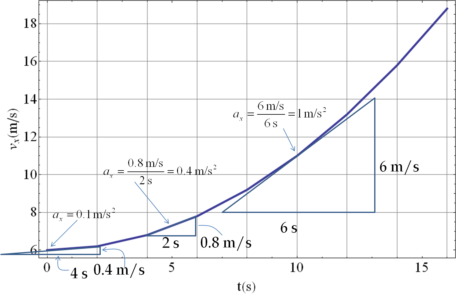
A motion detector is used to measure the velocity of a cart that moves along a straight track. The data is recorded as the \(x\)-component of the velocity by placing the \(x\)-coordinate on the track. The recorded \(x\)-component of the velocity is shownTable 2.52. Plot the data, and, from the graph, determine the acceleration at the following instants:(i) \(t =0\text{,}\) (ii) \(t = 5\) sec, and (iii) \(t = 10\) sec.
Table 2.52. Data from a Motion Detector for Exercise 2.5.5.1.
\(t(\text{s})\) \(v_x(\text{m/s})\) \(t(\text{s})\) \(v_x(\text{m/s})\)
0 6.0 10 11.0
2 6.2 12 13.2
4 6.8 14 15.8
6 7.8 16 18.8
8 9.2
Hint.
Find accelerations from a plot of velocity versus time.
Answer.
\(a_x(0) = 0.1\ \text{m/s}^2\text{,}\) \(a_x(5\ \text{s}) = 0.4\ \text{m/s}^2\text{,}\) \(a_x(10\ \text{s}) = 1\ \text{m/s}^2\text{.}\)
Solution.
Let’s plot \(v_x\) versus \(t\) as in Figure 2.53. The figure shows the calculations of the \(x\)-component of the acceleration. The acceletation at \(t=0\) is \(a_x(0) = 0.1\ \text{m/s}^2\text{,}\) at \(t=5\) s is \(a_x(5\ \text{s}) = 0.4\ \text{m/s}^2\text{,}\) and at \(t=10\) s is \(a_x(10\ \text{s}) = 1\ \text{m/s}^2\text{.}\)
Figure 2.53. Exercise 2.5.5.1.

2. Practice with a Friend : Analyze the Experiment.

The position of a glider on a straight track is determined at various times. The \(x\)-coordinate of the glider at various times is shown in Table 2.54. (a) From the given table or a plot of \(x\) vs \(t\) from the data in the table, determine the instantaneous velocities at sufficient number of instants [10 may be enough] to draw a smooth curve for the \(v_x\) vs \(t\) plot. (b) Draw the \(v_x\) vs \(t\) plot from the data generated in part (a). (c) From the \(v_x\) vs \(t\) plot you generated, estimate the values of the instantaneous acceleration at the following instants: (i) \(t = 2\) sec, (ii) \(t = 8\) sec, and (iii) \(t = 16\) sec.
Note the plots in this exercise are not necessarily smooth.
Table 2.54. Data from a Motion Detector for Exercise 2.5.5.2.
\(t(\text{s})\) \(x(\text{m})\) \(t(\text{s})\) \(x(\text{m})\)
0 0 9 -3
1 5 10 -35
2 10 11 -35
3 15 12 -32
4 20 13 -26
5 25 14 -17
6 25 15 -5
7 23 16 10
8 15

3.

4. (Calculus) Practice with a Friend.

The position of a block on a spring along \(x\) axis is given by
\begin{equation*} x(t) = A\, cos(\omega\, t + \phi), \end{equation*}
where \(A\text{,}\) \(\omega\text{,}\) and \(\phi\) are constant. Show that its acceleration at an arbitrary instant \(t\) is given by
\begin{equation*} a_x = -\omega^2\, x(t). \end{equation*}
Hint.
Differentiate \(x\text{.}\)

5. (Calculus) Practice with a Friend.

The acceleration of a car at the start is changing with time, as given by the following function.
\begin{equation*} a(t) = 12.0\; t^2. \end{equation*}
The unit of acceleration is \(\text{m/s}^2\text{.}\) If the car starts from rest, how far will it go in \(3.0\text{ sec}\text{?}\) Place the motion of the car along \(x\) axis.
Hint.
Integrate \(a_x\text{,}\) then integrate again.
Answer.
\(81.0\text{ m}\text{.}\)