Superposition of Electric Potential

Section 31.4 Superposition of Electric Potential

Similar to electric field, electric potential also obeys a superposition principle. But unlike electric field, the sum of two potentials is just an algebraic sum and not a vector sum. That makes working with potentials a much easier task.

Let’s say, some charge \(q_1\) has potential \(\phi_1\) at space point P and some other charge \(q_2\) has potential \(\phi_2\) at the same point P. Then, you would observe net potential at P to be just a simple sum of the two.

\begin{equation} \phi = \phi_1 + \phi_2.\tag{31.11} \end{equation}

It is easy to write a general formula for electic potential of a collection of \(N\) charges. Suppose the field point P is at distances \(r_1\text{,}\) \(r_2\text{,}\) \(r_3\text{,}\) \(\cdots\text{,}\) \(r_N\) from point charges \(q_1\text{,}\) \(q_2\text{,}\) \(q_3\text{,}\) \(\cdots\text{,}\) \(q_N\text{,}\) respectively. Superposition will give the net potential from all \(N\) charges.

\begin{align*} \phi_P \amp = \phi_1 + \phi_2 + \cdots + \phi_N,\\ \amp = \dfrac{1}{4\pi\epsilon_0}\, \left( \dfrac{q_1}{r_1} + \dfrac{q_2}{r_2} + \cdots + \dfrac{q_N}{r_N}\right) \\ \amp = \dfrac{1}{4\pi\epsilon_0}\, \sum_{i=1}^{N} \dfrac{q_i}{r_i}. \end{align*}

Note that the distances \(r_i\) between the charge and the field point P can be expressed in terms of the Cartesian coordinates of charge \(q_i\) and the field point. Let us denote the coordinates of P by \((x,\ y,\ z)\) and of charge \(q_i\) by \((x_i,\ y_i,\ z_i)\text{.}\) Then, we have

\begin{equation*} r_i = \sqrt{ (x-x_i)^2 + (y-y_i)^2 + (z-z_i)^2 }. \end{equation*}

Example 31.14. Electric Potential and Electric Field of Charges at Three Corners of a Square.

Three equal charges are located at the corners of a square of side \(a\) as shown. (a) Find the electric potential at the fourth corner. (b) Find the electric field at the fourth corner.

Answer.

(a) \(\dfrac{1}{4\pi\epsilon_0}\,\left( 2 + \dfrac{1}{\sqrt{2}} \right)\, \dfrac{q}{a} \text{.}\) (b) Magnitude \(E=k \dfrac{q}{a^2} \left( \sqrt{2} + \dfrac{1}{2}\right)\) in the diagonal direction.

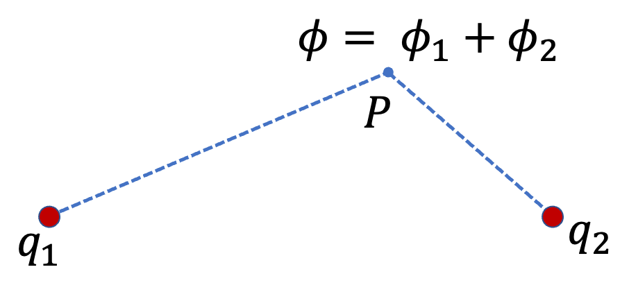
Solution 1. (a)

We just add up the potentials of the three charges.

\begin{align*} \phi_P \amp = \dfrac{1}{4\pi\epsilon_0} \left( \dfrac{q}{a} + \dfrac{q}{a\,\sqrt{2}} + \dfrac{q}{a}\right) \\ \amp = \dfrac{1}{4\pi\epsilon_0}\,\left( 2 + \dfrac{1}{\sqrt{2}} \right)\, \dfrac{q}{a}. \end{align*}

Solution 2. (b)

For electric field, let us assume the given charges are positive. We now need to include the impact of directions of the forces.

Let \(x\) axis be horizontal to the right and \(y\) vertically up. Let us also use \(k\) for \(1/4\pi\epsilon_0 \text{.}\) Then, we get the following for the magnitudes of the electric fields.

\begin{align*} E_1 \amp = k \dfrac{q}{a^2}\\ E_2 \amp = k \dfrac{q}{2a^2}\\ E_3 \amp = k \dfrac{q}{a^2} \end{align*}

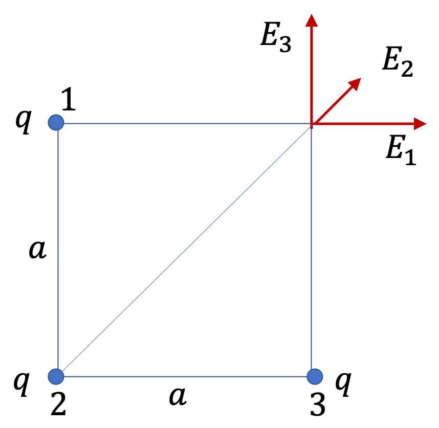
Note that net \(E\) at P is not just a simple sum of these.

\begin{equation*} E \ne E_1 + E_2 + E_3. \end{equation*}

We need to add them vectorially. This is simple enough to see that the magnitude of the field will be (we can get the same by working out the components, if you like)

\begin{align*} E \amp = E_1\,\cos\,45^\circ + E_3\,\cos\,45^\circ + E_2, \\ \amp = k \dfrac{q}{a^2} \left( \dfrac{1}{\sqrt{2}} + \dfrac{1}{\sqrt{2}} + \dfrac{1}{2}\right), \\ \amp = k \dfrac{q}{a^2} \left( \sqrt{2} + \dfrac{1}{2}\right), \end{align*}

and the direction is \(45^\circ\) in the direction of \(\vec E_2\text{.}\)