Section 13.1 Sine and Cosine Functions
You have seen sines and cosines in the context of triangles. There, we define them using the sides of a right-angled triangle which we have used when we studied vectors.

\begin{align*}
\amp \sin\,\theta = \dfrac{p}{h}, \\
\amp\cos\,\theta = \dfrac{b}{h}.
\end{align*}
Right-angles triangle only allows us to define the values of sines and cosines for values of the angle between zero and \(90^\circ\) or \(\pi/2\) radian. In many context we want sine and cosine for any real value of \(\theta\text{.}\) For that, unit circle-based definition of sine and cosine functions is perhaps most appropriate.
A unit circle is a circle with radius \(1\) (no units) as in Figure 13.1, which means the circumference is \(2\pi\text{.}\) The Cartesian coordinates on the unit circle gives cosine and sine of the angle subtended with the positive \(x\)-axis at the center since \(h=1\text{,}\) \(p=y\text{,}\) and \(b=x\) in the right-angled triangle shown.
\begin{align*}
\amp \cos\theta = x\\
\amp \sin\theta = y
\end{align*}

From the equation of unit circle
\begin{equation*}
x^2 + y^2 = 1,
\end{equation*}
and \(x=\cos\theta\) and \(y=\sin\theta\) on unit circle, we immediately get the following useful relation between sines and cosines.
\begin{equation}
\sin^2\theta + \cos^2\theta = 1.\tag{13.1}
\end{equation}
With radius \(r=1\text{,}\) angle \(\theta\) equals the arc length due to \(\theta = s/r = s\text{.}\) The angle given by arc length of unit circle is radians. With circumference of unit circle \(C=2\pi r = 2\pi\text{,}\) when you go around the circle, you cover and angle of \(2\pi\) radians with \(\theta = 2\pi\) radians same point on the circle as \(\theta = 0\text{.}\) That is,
\begin{equation*}
0 \le \theta \lt 2\pi.
\end{equation*}
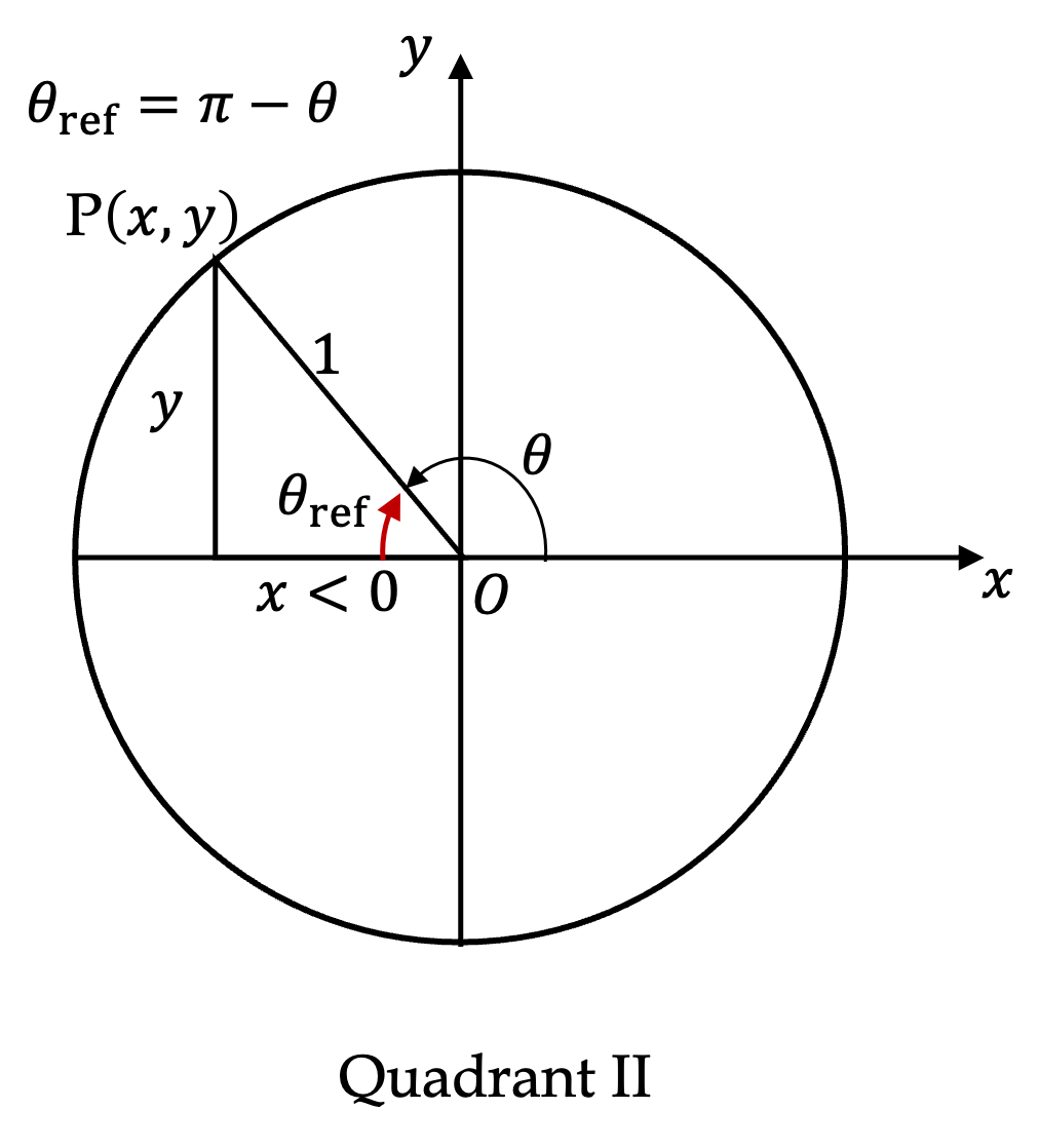
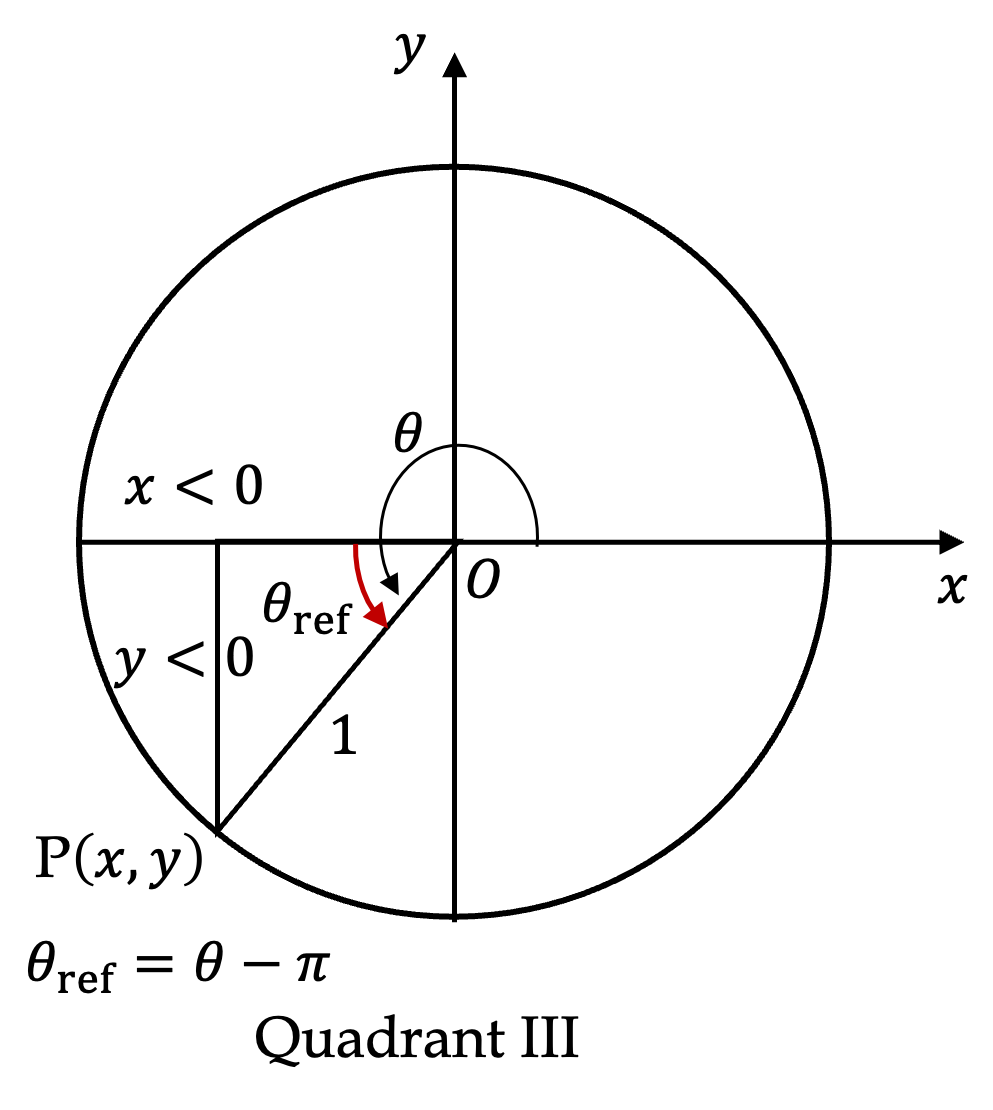
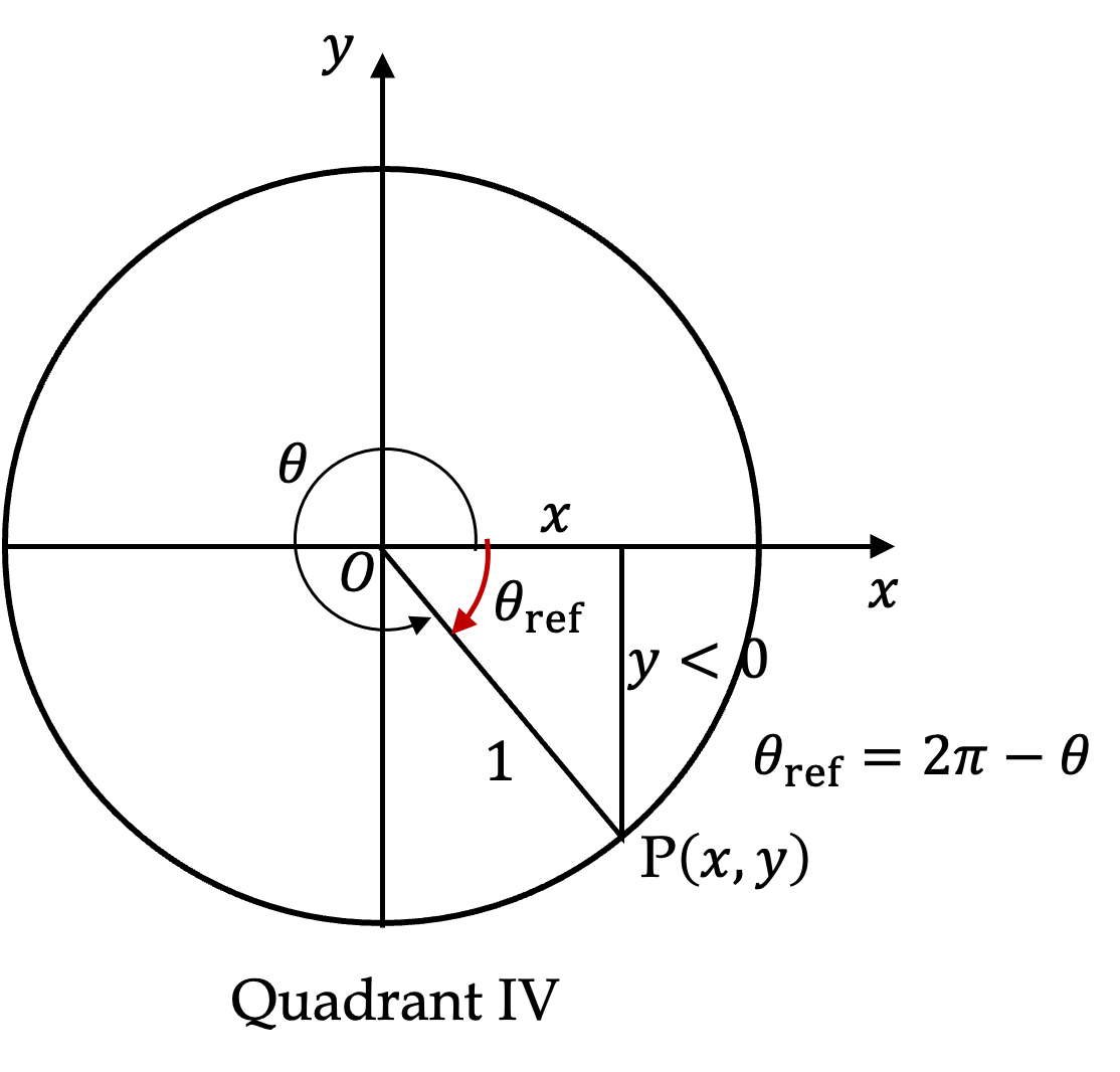
The definition shown for the first quadrant in Figure 13.1 extends to arbitrary point on the unit circle in all other quadrants as long as we measure the angle with resspect to the positive \(x\)-axis as shown in Figure 13.2. In 2nd, 3rd, and 4th quadrants, often we use a reference angle, \(\theta_\text{ref}\) to denote the direction.

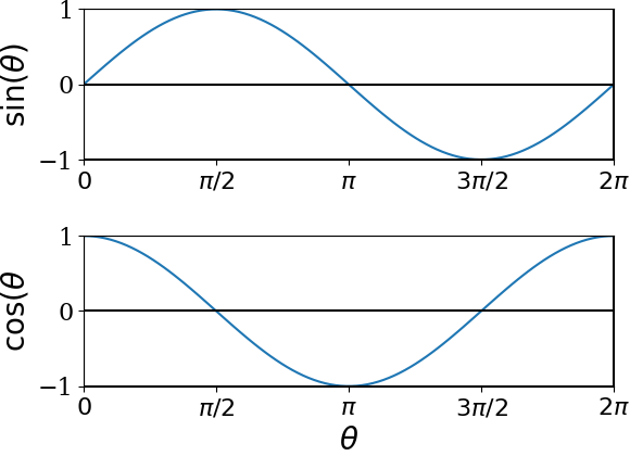
Clearly, sines and cosine functions are periodic functions with period \(2\pi\) radians. Using this periodicity, sines and cosine of any real number radians will map into a value of sine and cosine in the primary domain \(0\le \theta\lt 2\pi\text{.}\) Therefore, it is sufficient to plot sine and cosine in a primary domain as shown in Figure 13.3. Actually, you can pick any domain of length \(2\pi\text{,}\) e.g., sometimes it is more convenient to use \(-\pi\lt \theta \le \pi\) as the primary range.
\begin{align*}
\amp \sin\,(\theta + 2\pi m) = \sin\,\theta, \ \ \ (m\text{ any integer}) \\
\amp\cos\,(\theta + 2\pi n) = \cos\,\theta, \ \ \ (n\text{ any integer})
\end{align*}
This periodicity of sine and cosine functions makes them valuable for representing vibrations and waves, such as sound and light.