Kirchhoff’s Rules

Section 34.9 Kirchhoff’s Rules

When a circuit has only one power source, it can often be analyzed by constructing an equivalent circuit by successively employing series-parallel-series-etc to the circuit elements. If the circuit has more than one power source in different branches, or if employing series-parallel-series-etc method becomes too difficult or impossible to carry out, we appeal to the conservation principles of charge and energy in the circuit. These conservation principles lead to two rules called the Kirchhoff’s rules or the Kirchhoff’s laws.

The Node Rule or Kirchhoff’s current law (KCL)

In a circuit, charges do not accumulate or deplete from any point - any charge leaving a point by way of an outgoing current is replenshed by charges arriving by way of incoming current. The rate of leaving and arrival must equal due to the principle of conservaiton of charge.

Suppose we represent current comming to a point by a positive number and that leaving by a negative number, then we will find that sum of incoming and outgoing currents must equal zero (Figure 34.52). That is, algebraic sum of all currents must be zero.

\begin{equation} \sum I = 0.\tag{34.37} \end{equation}

When we apply this law to nodes of a circuit, we get relations among currents in various branches of the circuit.

The Loop Rule or Kirchhoff’s voltage law (KVL)

Suppose we start at an arbitrary point in an electric circuit and move an arbitrary charge $q$ on the circuit through various circuit elements, finally arriving at the initial place, thus making a closed loop. Since final place is same as the initial place, net change in energy of the charge will be zero. To go across some elements, you would need to put in energy; in some other place you would have to take away energy from $q\text{,}$ making the net change zero.

\begin{equation*} \sum_\text{steps across elements} U = 0. \end{equation*}

Since potentials across circuit elements are usually different, when you go across an element, the energy of the charge goes up or goes down by $q\Delta\phi\text{,}$ goes up if $\Delta\phi \gt 0$ and goes down if $\Delta\phi \lt 0\text{.}$ These increases and decreases must sum to zero as illustrated in Figure 34.53.

Figure 34.53. Kirchhoff’s voltage law or the loop rule: $\sum_\text{around a loop} \Delta\phi= 0\text{.}$

Since $q $ is a common factor in this sum, we can just sum potential differences in each step and the sum should equal zero.

\begin{equation} \sum_\text{around a loop} \Delta\phi= 0.\tag{34.38} \end{equation}

This is the loop rule or Kirchhooff’s voltage law (KVL). Applying this law to loops in circuits gives us relations among the potential values $\phi_i$ at various nodes of the circuit. These potential values are sometimes also called voltage values at those points - these values are potential difference with respect to a point chosen to be zero of the potential, which is usually the negative of some power source.

Subsection 34.9.1 Sign Conventions for Voltage in Loop Equation

To apply the Kirchhoff’s Loop Rule, it is often helpful to follow a sign convention for currents and voltages for consistency in algebraic manipulations. While electric circuit is a fixed structure, Kirchhoff’s loop is arbitrary loop. Hence, the direction of voltages and currents in the actual circuit may differ from the way you traverse a particular Kirchhoff’s loop. Therefore, it is important that you maintain a sign convention that assigns increase or decrease in voltage consistently across all your calculations.

Sign Convention for Voltage Sources

For potentials across a voltage source, we note that potential drops from a higher value to a lower value when you go from the positive terminal of a battery to its negative terminal, but if you go in the other direction, the potential will increase across the battery. Therefore, when we go from the negative to the positive of a voltage source, the change in potential is positive and when we go from positive to the negative of the source the change in potential is negative as shown in Figure 34.54.

Figure 34.54. Sign convention for a voltage source.

Sign Convention for Voltages Across Resitors

Similarly, when we assume a direction of current in a resistor, we are actually assuming one side of the resistor as being at a higher potential than the other side since the current flows from the higher potential towards the lower potential.

In a circuit we may not know the direction of a current a-priori, but we must pick a direction in order to proceed in calculations. Therefore, we label the two ends of a resistor with $+$ and $-$ to indicate the sides presumed to be at higher and lower voltages respectively. Although such labeling is not necessary but it often helps avoid silly mistake. This is illustrated in Figure 34.55.

Figure 34.55. Using sign convention shows that voltage drop across can be $+IR$ or $-IR$ depending upon the direction of traversal in the Kirchhoff’s voltage loop.

Zero Voltage Reference in a Circuit with Multiple Voltage Sources

When you have multiple voltage sources in a circuit, you can choose the negative end of only one of the sources. The negative ends of only those sources which are directly connected to the zero potential chosen will be at zero potential. The voltage of the source tells us by how much potential changes when you go across from the negative end to the positive end.

Subsection 34.9.2 Applying KCL and KVL

In a circuit with given resitors and voltage sources, there are two types of unknowns:

Currents through each circuit element, i.e., through each resistor and through each voltage source, or alternately, in each branch of the circuit.
Electric potential drop across each circuit element, i.e., across each resistor and across each voltage source.

From potential drops across every resistor we can us Ohm’s law to find current through them, and using KCL then lets us find current through the voltage sources. On the other hand, from current through each resistor, we can us Ohm’s law to find potential drops across each resistor.

Therefore, we can choose to set up algebraic quations for unknown currents or unknown potentials. Since current through all elements that are connected in series would be same, i.e., there is one current per branch rather than one current for each element, it is often easier to set up equations for currents. But if you are careful with potential drops, same amount of algebra is involved in that approach. In the end, it is up to you to see which way to proceed.

Example 34.56. Circuit With Two Voltage Sources.

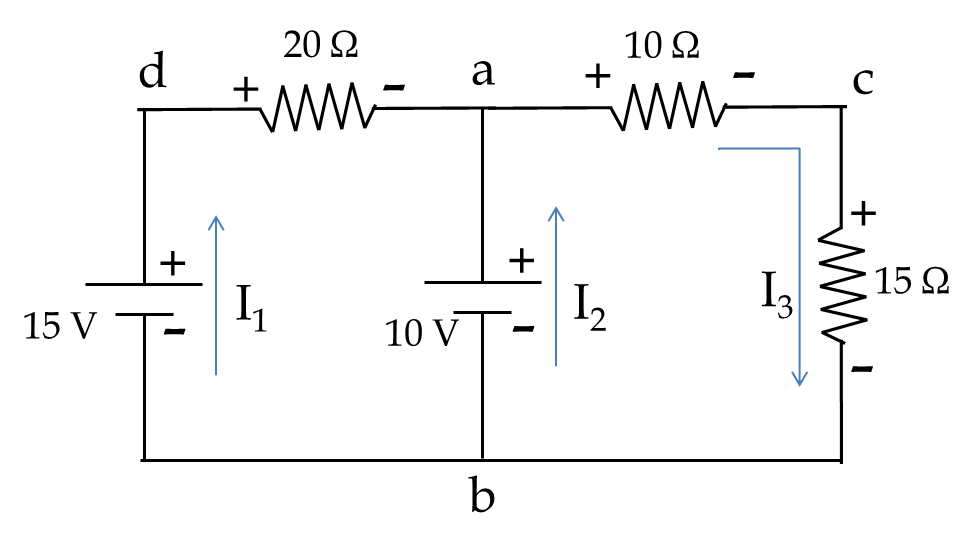
Find current through each resistor in the circuit in Figure 34.57. The values are: $R_1 = 10\ \Omega\text{,}$ $R_2 = 20\ \Omega\text{,}$ $R_1 = 30\ \Omega\text{,}$ $V_1 = 10\ \text{V}\text{,}$ $V_2 = 15\ \text{V}\text{.}$

Answer.

$I_1=\frac{1}{22}\, \text{ A},\ I_2=\frac{6}{22}\, \text{ A},\ I_3=\frac{7}{22}\, \text{ A}.$

Solution.

First we pick currents in each branch and label the resistors with $+$ and $-$ across each resistor based on our choice of direction of current as shown in Figure 34.58. Note that, at this stage I do not know the directions of the currents, but I must pick these directions based on intuition or arbitrarily.

The directions are then used to assign $+$ and $-$ across each resistor. These will be used to assign pick up voltage or drop off voltage in the Kirkchoof’s loop equations. We also recognize nodes where potential values are unique. There are four such nodes, labeled, $a\text{,}$ $b\text{,}$ $c\text{,}$ and $d\text{.}$

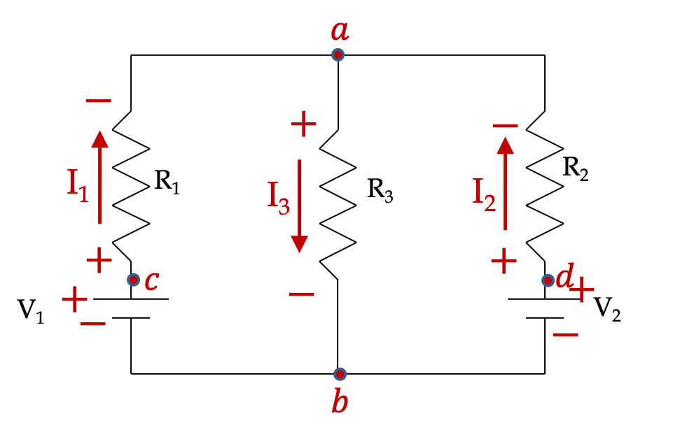
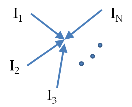
There are two junctions in the diagram where currents meets. We get the same KCL equation from them.

\begin{equation} I_1 + I_2 - I_3 = 0.\tag{34.39} \end{equation}

This gives us one equation in three unknowns. Therefore, we need to generate two other equations, which will come from KVL applied to two loops in the circuit.

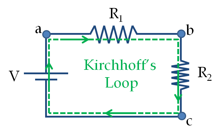
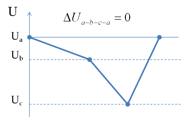
Let’s apply KVL in loop $a-b-c-a\text{.}$

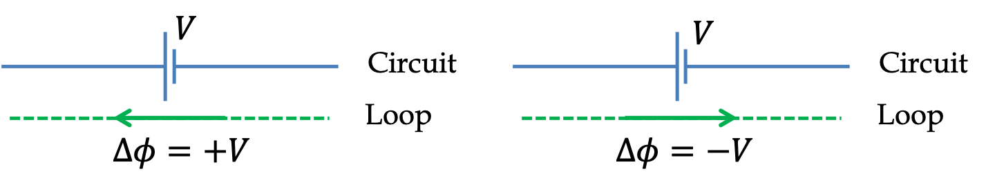
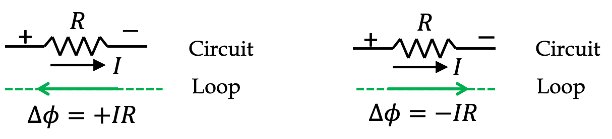
In the $a-b$ step, we are going in the same direction in the math loop as the current in the resistor. Therefore, the potential will drop by $I_3R_3\text{,}$ which is evident in going from $+\text{ to }-$ of the element. Then, in step $b-c\text{,}$ we go from $-\text{ to }+\text{,}$ which will mean increase of potential by $V_1\text{.}$

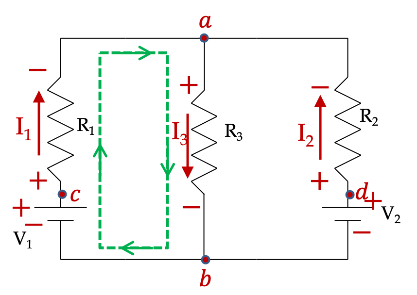
Finally, in step $c-a\text{,}$ we go from $+\text{ to }-\text{,}$ therefore, there will be a drop of potential of magnitude $I_1R_1\text{.}$ We get

\begin{equation*} -I_3R_3 + V_1 - I_1R_1 = 0. \end{equation*}

Using the numerical values we get

\begin{equation} -30 I_3 + 10 - 10 I_1 = 0.\tag{34.40} \end{equation}

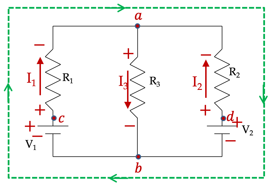
Finally, we apply KVL to the outer loop $a-d-b-c-a\text{.}$

In step $a-d$ we will have increase of $I_2R_2$ since, in the loop, we are going against the direction of the current in the resistor, or equivalently, we are going from $-\text{ to }+$ of the assigned signs to the resistor. In step $a-d\text{,}$ the potential drops by $V_2\text{.}$ In step $b-c\text{,}$ potential goes up by $V_1$ and in step $c-a\text{,}$ potential drops by $I_1R_1\text{.}$

Therefore,

\begin{equation*} +I_2R_2 -V_2 + V_1 - I_1R_1 = 0. \end{equation*}

Using the numerical values we get

\begin{equation} +20 I_2 -15 + 10 - 10 I_1 = 0.\tag{34.41} \end{equation}

You can solve Eqs. (34.39), (34.40), and (34.41) by method of elimination or some other method you are more familiar with. It is very common to make mistakes in these calculations, so, you should pluc back your answer into these equations to check your answer. I used the command “Solve x+y=z, 10x+30z=10, 10x -20y=-5” at Wolfram Alpha

website. My answers are

\begin{equation*} I_1=\frac{1}{22}\, \text{ A},\ I_2=\frac{6}{22}\, \text{ A},\ I_3=\frac{7}{22}\, \text{ A}. \end{equation*}

Since I got all of these current magnitude positive, my original directions were correct. If I had got any of them negative, it would tell me that the direction of the current I picked in the figure above should have been the oposite direction.

Example 34.61. Numerical Bridge Circuit Example.

In a bridge circuit, resistors and other elements in a circuit form a bridge-like structure. Bridge circuits are used for many purposes in engineering and physics. Find currents in each wire of the bridge circuit given in Figure 34.62.

Answer.

$I = \frac{78}{155}\, \text{ A}\text{,}$ $I_1 = \frac{51}{155}\, \text{ A}\text{,}$ $I_2 = \frac{27}{155}\, \text{ A},$ $I_3 = \frac{45}{155}\, \text{ A}\text{,}$ $I_4 = \frac{33}{155}\, \text{ A}\text{,}$ $I_5 = \frac{6}{155}\, \text{ A}.$

Solution.

Using current conservations at nodes we get three equations from four nodes, the KCL on the fourth node is just a sum of the other relations.

\begin{align} \amp \text{node a: } I = I_1 + I_2 \tag{34.42}\\ \amp \text{node b: } I_1 = I_3 + I_5\tag{34.43}\\ \amp \text{node d: } I_2 + I_5 = I_4\tag{34.44} \end{align}

These give us three relations among six unknowns, $I,\ I_1,\ I_2,\ I_3,\ I_4,\ I_5\text{.}$ Therefore, we need three loops equations from KVL. We can pick any three loop in the circuit. My choice is shown in figure below.

The KVL equations for the three loops are

\begin{align} \amp -10 I_1 - 5 I_5 + 20 I_2 = 0 \tag{34.45}\\ \amp -30 I_3 + 40 I_4 + 5 I_5 = 0\tag{34.46}\\ \amp -20 I_2 -40 I_4 + 12 = 0\tag{34.47} \end{align}

Solving Eqs. (34.42) to (34.47) simultaneously will give the values of the six currents in the circuit. You can systematically apply the method of elimination. Very tedious to do that. I will carefully type command at Wolfram Alpha

website. Here is the command I used, “Solve a = a1 + a2, a1 = a3 + a5, a2 + a5 = a4, -10 a1 - 5 a5 + 20 a2 = 0, -30 a3 + 40 a4 + 5 a5 = 0, -20 a2 - 40 a4 + 12 = 0,” which gave me the following answer.

\begin{align*} \amp I = \frac{78}{155}\, \text{ A}, I_1 = \frac{51}{155}\, \text{ A}, I_2 = \frac{27}{155}\, \text{ A},\\ \amp I_3 = \frac{45}{155}\, \text{ A}, I_4 = \frac{33}{155}\, \text{ A}, I_5 = \frac{6}{155}\, \text{ A}. \end{align*}

Example 34.63. Finding Electric Potentials in a Bridge Circuit.

In a bridge circuit, resistors and other elements in a circuit form a bridge-like structure. You can analyze the circuit given in Figure 34.64 by setting up six equations for six currents. That is not the most economical way for analyzing this circuit since it has only four unique values of electic potentials at four nodes in the circuit. The values of potentials at two of the nodes is already known. Therefore, we need to find only two unknown potentials. Find values of electric potential at the four nodes in the circuit.

Answer.

$\phi_a = 12\text{ V}\text{,}$ $\phi_b=0\text{,}$ $\phi_c = \frac{270}{31}\text{ V}\text{,}$ $\phi_d = \frac{264}{31}\text{ V}\text{.}$

Solution.

Let $\phi_a\text{,}$ $\phi_b\text{,}$ $\phi_c\text{,}$ and $\phi_d$ denote electric potentials at $a,\ b,\ c,\ d$ respectively. Since voltage source maintains potential difference across it,

\begin{equation*} \phi_a - \phi_b = 12\text{ V}. \end{equation*}

We can always, choose one place to be zero reference of electric potential. As customary, we will choose it to be the negative of a voltage source. Note, if we had multiple voltage sources, negative of only one of them can be set to zero.

\begin{equation*} \phi_b = 0,\ \phi_a= 12\text{ V}. \end{equation*}

From the circuit we have the following for Ohm’s law for each resistor.

\begin{align*} \amp 12- \phi_c = 10 I_1\\ \amp 12- \phi_d = 20 I_2\\ \amp \phi_c -0 = 30 I_3\\ \amp \phi_d -0 = 40 I_4\\ \amp \phi_c - \phi_d = 5 I_5 \end{align*}

We will use these to replace currents in the following KCL equations at nodes $c$ and $d\text{,}$

\begin{align*} \amp I_1 = I_3 + I_5,\\ \amp I_4 = I_2 + I_5, \end{align*}

which gives

\begin{align*} \amp \frac{12-\phi_c}{10} = \frac{\phi_c}{30} + \frac{\phi_c - \phi_d}{5},\\ \amp \frac{ \phi_d}{40} = \frac{12-\phi_d}{20} + \frac{\phi_c - \phi_d}{5}. \end{align*}

These can be simplified to

\begin{align*} \amp 10 \phi_c - 6 \phi_d = 36,\\ \amp -8 \phi_c + 11 \phi_d = 24. \end{align*}

Solving them yields

\begin{equation*} \phi_c = \frac{270}{31}\text{ V},\ \ \phi_d = \frac{264}{31}\text{ V}. \end{equation*}

From the potentials, it is trivial to get the currents now.

Exercises 34.9.3 Exercises

1.

Find current in all branches in the circuit in Figure 34.65.

Answer.

$0.15\, \text{A}\text{,}$ $0.25\, \text{A}\text{,}$ $0.4\, \text{A}\text{.}$

Solution.

Step 1: Choose (arbitrary) current directions in the circuit. There are three branches in the circuit. Let $I_1\text{,}$ $I_2$ and $I_3$ denote currents in them. We assign the direction in the Figure pretty much arbitrarily. After the solution, we shall know the actual direction.

Step 2: Assign $+$ and $-$ to each resistor. Using the assumed direction of current it is convenient to label $+$ and $-$ across each resistor. The labeling of $+$ and $-$ across voltage sources is not dependent on the current direction since the voltage source have innate polarity.

Step 3: Label node points and other points so that we have ways to uniquely refer to loops. We need only label four points for the given circuit, labeled a, b, c and d.

Step 4: Generate Kirchoff’s equations. There should be as many independent equations as there are unknowns.

Node equations: Since there are two nodes, we get only one independent equation.

\begin{equation*} I_1 + I_2 - I_3 = 0. (1) \end{equation*}

Loop equations: Since there are three unknown currents, and only one node equation, we must generate two loop equations. Although there are three loops possible in the diagram, we may choose any two. I will choose a-b-d-a and a-b-c-a.

\begin{align*} \amp \text{a-b-c-d:}\ \ \ \ -10 + 15 - 20 I_1 = 0\ \ \ (2)\\ \amp \text{a-b-c-a:}\ \ \ \ -10 + 15 I_3 + 10 I_3 = 0\ \ \ (3) \end{align*}

Pay particular attention to pluses and minuses in equations (1), (2) and (3).

Step 5: Solve for the currents. From (2) we get $I_1 = 0.25\:\text{A}\text{,}$ and from (3) we get $I_3 = 0.25\:\text{A}\text{.}$ Put these in (1) to obtain $I_2 = 0.15\:\text{A}\text{.}$

Since all the currents turned out to be positive, the actual currents are in the same direction as selected in the figure. Just a lucky break!

2.

Ten watts of power is desired in the $8\, \Omega$ resistor in circuit shown in Figure 34.67. What voltage should be applied by source labeled A.

Answer.

$21\,\text{V}\text{.}$

Solution.

Let us redraw the circuit with the current in the three branches labeled as in Figure 34.68.

From the power delivered to the eight Ohm resistor, we know the magnitude of the current in that branch.

\begin{equation*} I_1 = \sqrt{\frac{P}{R}} = \sqrt{\frac{10}{8}} = 1.118\:\text{A}. \end{equation*}

We can write the Kirchhoff’s equations from one independent node and two independent loops.

\begin{align*} \amp \text{Current equation:}\ \ 1.118 - I_2 - I_3 = 0.\\ \amp \text{Loop equation, V-8-12-V:}\ \ -12\:\text{V} + V - 8 \times 1.118 = 0.\\ \amp \text{Loop equation, 12-6-2-12:}\ \ 12\:\text{V} - 6 I_3 - 2 I_3 = 0. \end{align*}

Therefore, $V = 21\:\text{V}\text{.}$

3.

Find the voltage drop across $2500\,\Omega$ resistor in Figure 34.69.

Answer.

$(175/8)\, \text{V}\text{.}$

Solution.

There are six branches now, therefore there will be six currents as shown in the figure below.

Three independent node equations:

\begin{align*} \amp - I_1 - I_4 + I_5 = 0,\\ \amp I_1 - I_2 + I_3 = 0,\\ \amp I_4 + I_2 + I_5 = 0. \end{align*}

Three independent loop equations:

\begin{align*} \amp 10 + 1200 I_4 - 1500 I_1 = 0,\\ \amp 10 - 2000 I_5 - 2500 I_3 = 0,\\ \amp 15 - 1500 I_1 + 2500 I_3 = 0. \end{align*}

Perhaps the easiest way to handle six linear equations in six unknowns is to organize the data in a matrix form and use a calculator.

\begin{equation*} \left[ \begin{array}{cccccc} -1 \amp 0 \amp 0 \amp -1 \amp 0 \amp 1 \\ 1 \amp -1 \amp 1 \amp 0 \amp 0 \amp 0 \\ 0 \amp 1 \amp 0 \amp 1 \amp 1 \amp 0 \\ 1500 \amp 0 \amp 0 \amp 1200 \amp 0 \amp 0 \\ 0 \amp 0 \amp -2500 \amp 0 \amp -2000 \amp 0 \\ -1500 \amp 2500 \amp 0 \amp 0 \amp 0 \amp 0 \end{array} \right] \left[ \begin{array}{c} I_1\\ I_2\\ I_3\\ I_4\\ I_5\\ I_6 \end{array} \right] = \left[ \begin{array}{c} 0\\ 0\\ 0\\ -10\\ -10\\ -15 \end{array} \right] \end{equation*}

We find the following values for currents.

\begin{align*} \amp I_1 = - \frac{11}{2400}\:\textrm{A},\ \ I_2 = -\frac{1}{75}\:\textrm{A},\ \ I_3 = -\frac{7}{800}\:\textrm{A},\\ \amp I_4 = - \frac{1}{384}\:\textrm{A},\ \ I_5 = \frac{51}{3200}\:\textrm{A},\ \ I_6 = -\frac{23}{3200}\:\textrm{A}. \end{align*}

Therefore, the voltage drop across the $2500\,\Omega$ resistor is

\begin{equation*} V = \frac{7}{800}\times 2500 = \frac{175}{8}\:\textrm{V}. \end{equation*}

Prev Top Next