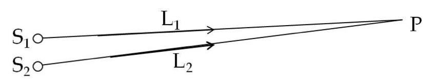
This experiment can be set up, for example, by having two slits in a plate through which waves must exit on the other side and move to \(P\) where they must produce a net vibration. For instance, we can shine light from a laser on an opaque plate with two slits at \(S_1\) and \(S_2\text{.}\) The experimental arrangement with two slits is also called Young’s double slit experiment who studied interference of light waves by this method.
Even if the two waves start out in sync at
\(S_1\) and
\(S_2\text{,}\) they might not be in sync at point
\(P\) on the screen, depending upon relative distances from the source points to
\(P\text{.}\) If the difference between
\(L_1\) and
\(L_2\) is a multiple of a wavelength, then we expect them to end up in sync again at
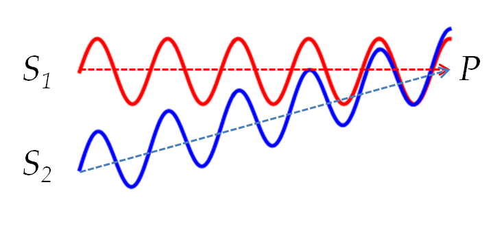
\(P\) and a maximum intensity should result there. When this happens, we say that the two waves have a constructive interference at point
\(P\text{.}\) This is shown in
Figure 14.31 where two waves which start out at points
\(S_1\) and
\(S_2\) in sync end up in sync at point
\(P\text{.}\)
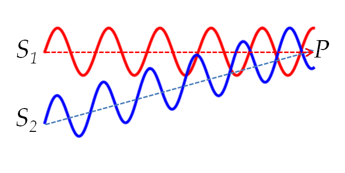
On the other hand, if the difference of distances from the sources at
\(S_1\) and
\(S_2\) to the point
\(P\) is an odd multiple of half a wavelength, then the crest of one wave will fall on the trough of the other, making the net amplitude zero there. The waves are said to interfere destructively at point
\(P\text{.}\) If the amplitudes of the waves from
\(S_1\) and
\(S_2\) are equal, then, the net amplitude at the point of destructive interference will be zero since the two waves will be completely out of sync there. This is shown in
Figure 14.32 where two waves which start out in sync at points
\(S_1\) and
\(S_2\) end up out of sync at point
\(P\) and interfere destructively there.
Let us now see how the constructive and destructive interferences show up analytically as a result of the addition of the amplitudes of the two waves. For this, we need to work out the interference term more fully.
\begin{equation*}
I_{12} = 2 \alpha \langle \psi_1 \psi_2 \rangle.
\end{equation*}
Since waves 1 and 2 travel distances \(L_1\) and \(L_2\) their wave functions at point \(P\) will take on the following values at an arbitrary time \(t\text{.}\)
\begin{align*}
\amp \psi_1(t) = A \cos\left(kL_1 - \omega t \right) \\
\amp \psi_2(t) = A \cos\left(kL_2 - \omega t \right)
\end{align*}
Note the waves have the same frequency, wavenumber and amplitude for our exercise here. Note also that we have dropped the phase constant since we have assumed that the waves start out in sync at \(S_1\) and \(S_2\text{.}\) Multiplying the two wave functions we find
\begin{align*}
\psi_1(t)\psi_2(t) \amp = A^2 \cos\left(kL_1\right)\cos\left(kL_2\right) \cos^2\omega t \\
\amp \ \ \ + A^2 \sin\left(kL_1\right)\sin\left(kL_2\right) \sin^2\omega t\\
\amp \ \ \ - A^2 \cos\left(kL_1\right)\sin\left(kL_2\right) \cos\omega t \sin\omega t\\
\amp \ \ \ - A^2 \sin\left(kL_1\right) \cos\left(kL_2\right) \cos\omega t \sin\omega t
\end{align*}
We need to find time-average of this. That involved calculating time averages, \(\langle \cos^2\omega t rangle\text{,}\) \(\langle \sin^2\omega t rangle\text{,}\) and \(\langle \cos\omega t \sin\omega t rangle\text{.}\) The time average of a periodic function can be easily done by an integration over one period and dividing by the period. Let \(T\) be the period.
\begin{equation}
\langle f(t) \rangle = \frac{1}{T}\int_0^T f(t) dt. \tag{14.74}
\end{equation}
By using this definition, we get
\begin{align}
\amp \langle \cos^2(\omega t)\rangle = \frac{1}{T}\int_0^T \cos^2(\omega t) dt = \frac{1}{2}\tag{14.75}\\
\amp \langle\sin^2(\omega t)\rangle = \frac{1}{T}\int_0^T \sin^2(\omega t) dt = \frac{1}{2}\tag{14.76}\\
\amp \langle \cos(\omega t)\sin(\omega t)\rangle = \frac{1}{T}\int_0^T \cos(\omega t)\sin(\omega t) dt = 0\tag{14.77}
\end{align}
Therefore, the interference term evaluates to
\begin{equation*}
I_{12} =\alpha A^2 \cos\left[k\left( L_1 -L_2 \right)\right].
\end{equation*}
Note the intensity of each wave is
\begin{equation*}
I_{1}= I_{2} \propto \langle \psi_1^2\rangle = \frac{1}{2}\alpha A^2.
\end{equation*}
Let us write the intensity of the individual waves as \(I_0\text{.}\)
\begin{equation*}
I_0 \equiv I_1 = I_2.
\end{equation*}
Now, writing the intensity observed at point P, all in terms of \(I_0\text{,}\) the intensity of separate waves, is
\begin{equation}
I = 2I_0\left\{ 1+ \cos\left[k\left( L_1 -L_2 \right)\right]\right\}\tag{14.78}
\end{equation}
For fixed source points \(S_1\) and \(S_2\text{,}\) the intensity depends upon the location of the observation point \(P\) since depending upon the value of \(k(L_1-L_2)\) the cosine function fluctuates between \(-1\) and \(1\text{.}\) When cosine is equal to \(-1\text{,}\) the intensity at \(P\) will be zero, and when cosine is \(+1\text{,}\) the intensity is four times as much as the intensity in each wave. Hence, we have the following conditions for constructive and destructive interference.
\begin{equation*}
k(L_1 - L_2) =
\begin{cases}
2n\pi \amp n = 0, \pm 1, \pm 2, \cdots \text{Constructive} \\
(2n+1)\pi \amp n = 0, \pm 1, \pm 2, \cdots \text{Destructive}
\end{cases}
\end{equation*}
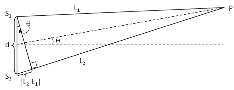
Let us write the wave number k in terms of the wavelength by using \(k = 2\pi/\lambda\text{,}\) we get a simpler form that clearly shows the path difference versus integral and half-integral multiples of wavelength.
\begin{equation*}
L_1 - L_2 =
\begin{cases}
n\lambda \amp n = 0, \pm 1, \pm 2, \cdots \text{Constructive} \\
\left( n + \frac{1}{2}\right)\lambda \amp n = 0, \pm 1, \pm 2, \cdots \text{Destructive}
\end{cases}
\end{equation*}
Therefore, the waves from two synchronized sources of the same frequency interfere constructively when the distances to an observation point \(P\) differ by multiples of a wavelength and interfere destructively if the distances differ by half a wavelength, or odd multiples of half a wave length.