Dynamics of Rigid Bodies

Section 10.4 Dynamics of Rigid Bodies

(Calculus) Motion of a rigid body has two aspects: (1) the translation motion of the center of mass and (2) the orientation of the body. For rigid bodies, the equations of motion from applying Newton’s second law of motion to every particle of the body separates into equations of motion of the center of mass of the body and equations of motion for angles that can be used to tell the orientation. In total, rather than having many equations of motion, three for each point of the body, we end up with only three equations of motion for the \(x_\text{cm}\text{,}\) \(y_\text{cm}\) and \(z_\text{cm}\) of the CM and three equations for the angles, which could be Eueler’s angles as we discuss below.

We have seen previously that when we add up equations of motion of all parts of a body, the vector sum gives us the equations of motion of the center of mass, i.e., from \(d\vec p)i/dt = \vec F_i\) for particles \(i\) of the body, we get

\begin{equation} \frac{d\vec P_\text{cm}}{dt} = \sum\vec F_\text{ext},\tag{10.20} \end{equation}

where

\begin{equation*} \vec P_\text{cm} = \vec p_1 + \vec p_2 + \cdots, \end{equation*}

and right side is the vector sum of external forces acting on any part of the body.

Since angular momentum of each particle \(\vec l_i = \vec r_i \times \vec p_i\text{,}\) the rate of change of net angular momentum will be

\begin{align*} \frac{d\vec L}{dt} \amp = \frac{d\sum \vec l_i}{dt} = \frac{d}{dt} \sum \left( \vec r_i \times \vec p_i\right)\\ \amp = \sum \left( \vec v_i \times \vec p_i + \vec r_i \times \frac{d\vec p_i}{dt} \right) \end{align*}

Here, first term will be zero since \(\vec v_i\) is parallel to \(\vec p_i\text{.}\) Using Newton’s second law for the second term we get

\begin{equation} \frac{d\vec L}{dt} = \sum \vec r_i \times \vec F_i.\tag{10.21} \end{equation}

The quantty \(\vec r_i \times \vec F_i\) is called moment of force \(\vec F_i\) about origin \(O\) with respect to which \(\vec r_i\) is the position of particle i. The sum of moments of all forces is called net torque on the body, which we denote by \(\vec{\mathcal{T}}\text{.}\)

\begin{equation} \frac{d\vec L}{dt} = \vec{\mathcal{T}}.\tag{10.22} \end{equation}

Equations (10.20) and (10.22) are with respect to inertial or fixed coordinate system. When axis of rotation is not fixed, rotation part is simpler when handled in the moving coordinate system, which can be setup to take advantage of symmetry of the body. Transforming between the two coordinate systems is a challengin exercise which we will tackle in a separate section. In this section we will examine simpler situations where making use of moving coordinates is relatively easy.

A fruitful way to apply (10.22) is to think (10.22) for small time duration. The change in angular momentum \(\Delta \vec L\) will be

\begin{equation*} \Delta \vec L = \vec L(t+\Delta t) - \vec L(t). \end{equation*}

Then, we can relate the change to torque to the change in angular momentum vector.

\begin{equation*} \vec{\mathcal{T}} = \frac{\vec L(t+\Delta t) - \vec L(t)}{\Delta t},\ \ \ \text{or}\ \ \ \Delta \vec L = \vec{\mathcal{T}}\, \Delta t. \end{equation*}

If magnitude of angular momentum is not changing, then Figure 10.34 shows that in the limit \(\Delta t\rightarrow 0\) limit, \(\vec L(t)\) and \(\vec L(t+\Delta t)\) are radial with tips at the circle of radius \(|\vec L|\) and therefore, \(\Delta \vec L\) is tangential. That would make \(\Delta\vec L\) perpendicular to \(\vec L\text{.}\)

Example 10.35. (Calculus) Torque on Rotating Angular Momentum of a Dumbbell.

In Example 10.15 we found angular momentum vector of a rotating dumbbell.

\begin{align*} \amp L_x = b \cos\omega t,\\ \amp L_y = b \sin\omega t,\\ \amp L_z = 2ma^2\sin^2\theta, \end{align*}

where \(b = 2m\omega a^2\sin\theta\cos\theta\text{.}\) (a) Show that projection of anglar momentum vector in \(xy\)-plane rotates about \(z\)-axis with angular speed \(\omega\text{.}\) (b) Some frce must be acting on the dumbbell for angular momentum vector to change in time. Find the torque on the dumbbell.

Answer.

(b) \(\mathcal{T}_x = - b\omega\, \sin\omega t,\ \ \mathcal{T}_y = b\omega\, \cos\omega t,\ \ \mathcal{T}_z=0\text{.}\)

Solution 1. a

The projection vector \(\vec L_{xy}\) at instant \(t\) will have components \(L_x\) and \(L_y\text{.}\) Projection vector is pointed in \(xy\)-plane radially out from the origin in the direction of angle \(\phi=\omega t\) with respect to \(x\)-axis. Therefore, this vector will rotate with angular speed \(\omega\text{.}\)

Solution 2. b

We apply rotational dynamics equation in the component form to get

\begin{align*} \amp \mathcal{T}_x = \frac{dL_x}{dt} = - b\omega \sin\omega t,\\ \amp \mathcal{T}_y = \frac{dL_y}{dt} = b\omega \cos\omega t,\\ \amp \mathcal{T}_z = \frac{dL_z}{dt} = 0. \end{align*}

Example 10.38. (Calculus) Torque on Rotating a Spinning Sphere.

Figure 10.39 shows a person holding the axle of a spinning sphere of mass \(M\) and radius \(R\) that is rotating about the axle at angular speed \(\omega\text{.}\) For simplicity, imagine this is in outer space. He starts to change the orientation of the axle at a steady angular speed \(\Omega\) by applying a steady torque. Find the torque required.

Answer.

\(\frac{2}{5}MR^2\omega\Omega\,\left( -\sin\Omega t\ \hat i + \cos\Omega t\ \hat j \right)\text{.}\)

Solution.

Let’s sketch a figure with axes for situation at instant \(t\text{,}\) when the axis is pointed in the direction with azimuthal angle \(\phi=\Omega t\text{.}\) Angular momentum from the spinning is denoted by \(\vec L_{xy}\) in the Figure 10.40.

Magnitude of \(\vec L_{xy}\) will be \(I\omega\) with \(I=\frac{2}{5}MR^2\) since axis is through the center of the sphere. Since \(\phi = \Omega\,t\text{,}\) the direction of \(\vec L_{xy}\) is that of unit vector \(\hat u\) given by

\begin{equation*} \hat u = \cos\Omega t\ \hat i + \sin\Omega t\ \hat j. \end{equation*}

Therefore, we will have

\begin{equation*} \vec L_{xy} = \frac{2}{5}MR^2\omega\,\left( \cos\Omega t\ \hat i + \sin\Omega t\ \hat j \right). \end{equation*}

The total angular momentum of the sphere will be

\begin{equation*} \vec L = \vec L_{xy} + \vec L_z, \end{equation*}

where \(L_z\) is the \(z\)-component of the angular momentum. Since \(L_z\) is constant in time, for torque we will get

\begin{align*} \vec{\mathcal{T}} \amp = \frac{d\vec L}{dt} = \frac{d\vec L_{xy}}{dt} \\ \amp = \frac{2}{5}MR^2\omega\Omega\,\left( -\sin\Omega t\ \hat i + \cos\Omega t\ \hat j \right). \end{align*}

Example 10.41. (Calculus) Torque on a Rolling Disk.

Figure 10.42 shows a disk of mass \(M\) and radius \(R\) attached to an axle of length \(a\) which is attached to a vertical rotatatable shaft. A torque \(\mathcal{T}\) is required to uniformly rotate the disk without slipping. Find required torque.

Answer.

\(\frac{1}{2}MR^2\omega\Omega\, \left(-\sin\Omega\,t \, \hat i + \cos\Omega\,t \, \hat j \right)\text{.}\)

Solution.

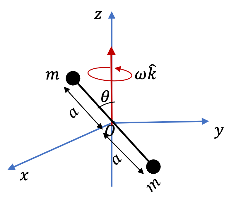
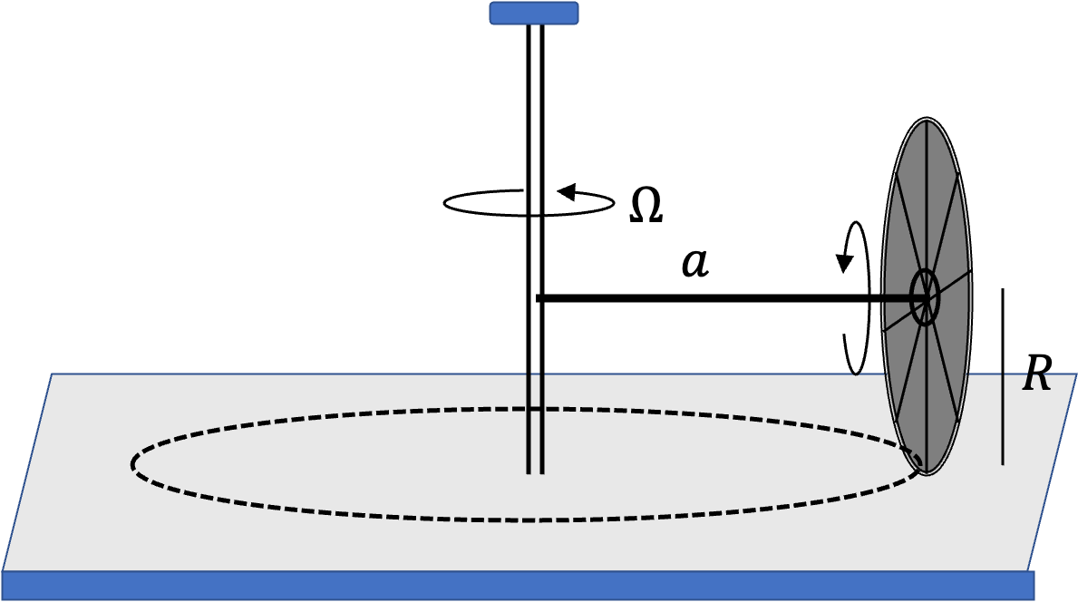
We can get speed of rotation of disk about the axle by noting that in the time \(\Delta t\) in which the disk goes once around in a circle of radius \(a\text{,}\) a point on the disk woould travel \(2\pi R n\) where \(n\) is the number of rotations. That is

\begin{equation*} 2\pi R n = 2\pi a. \end{equation*}

Therefore

\begin{equation*} n = a/R. \end{equation*}

We use angular speed for rolling around in circle of radius \(a\) to find time for going once around.

\begin{equation*} \Delta t = \frac{2\pi}{\Omega}. \end{equation*}

Therefore, angular speed for rotation about axle is

\begin{equation*} \omega = \frac{2\pi n}{\Delta t} = \frac{\Omega}{2\pi} \times \frac{ 2\pi a }{R} = \frac{a\Omega}{R}. \end{equation*}

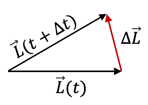
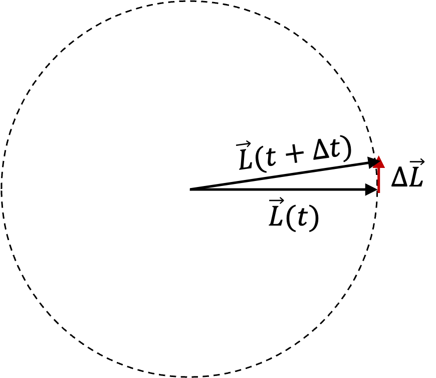
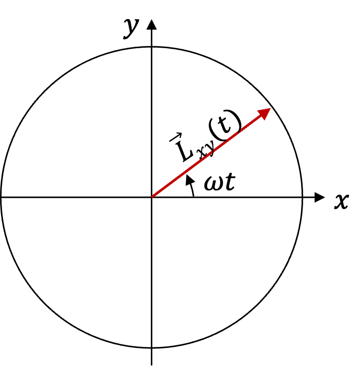
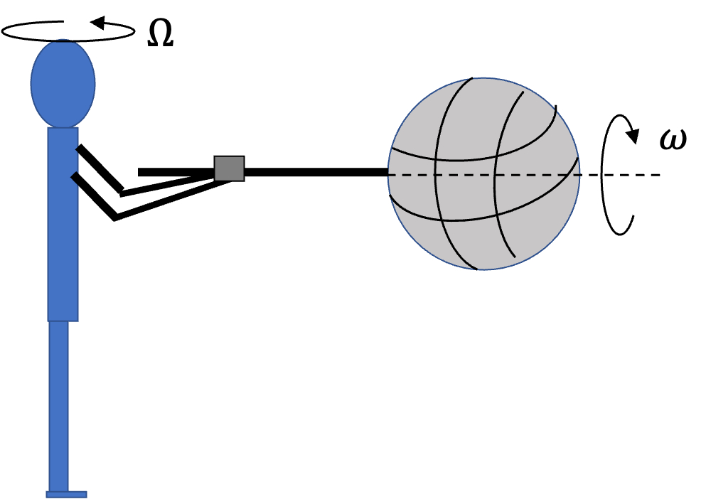
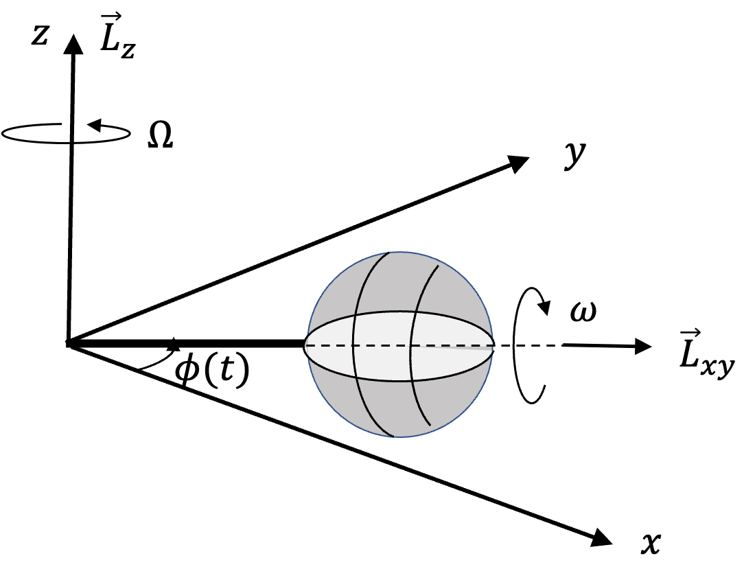
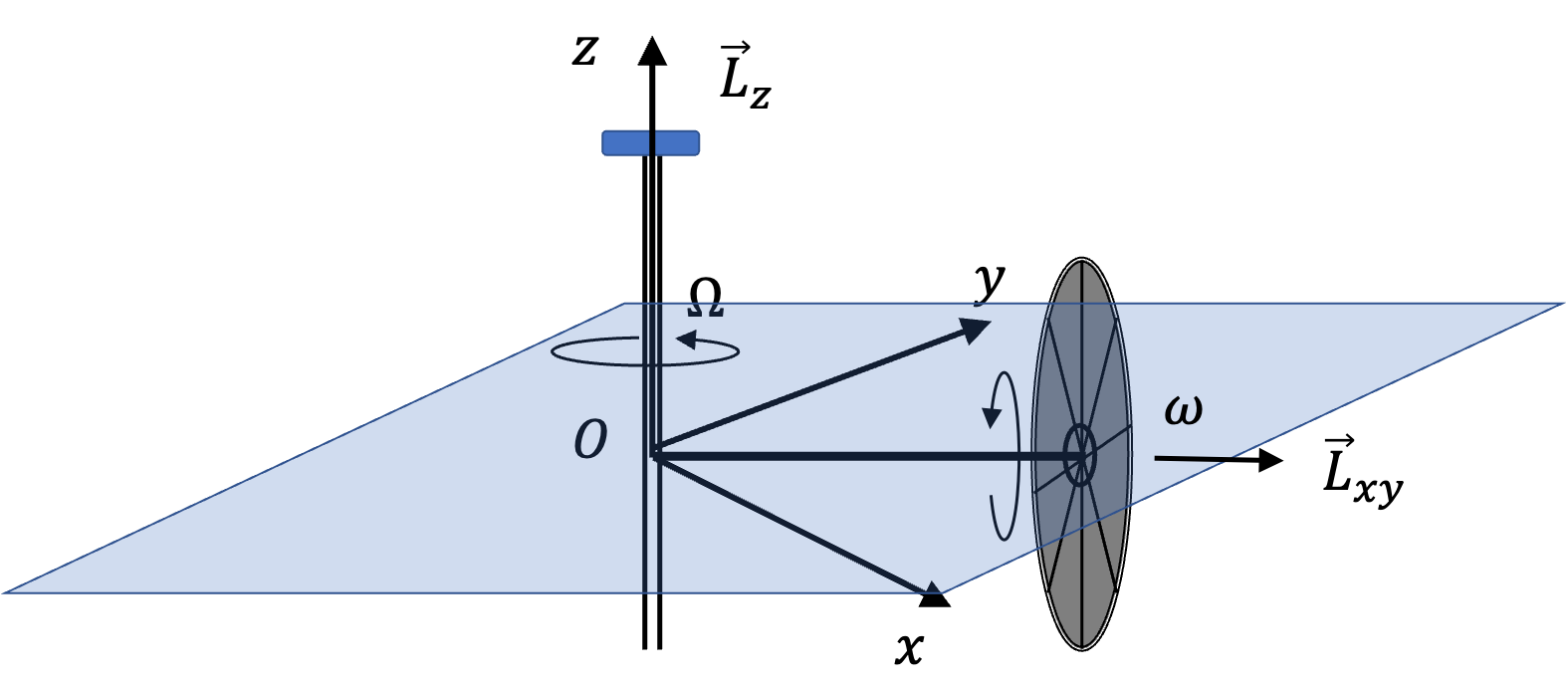
Since the disk is uniformly going around the central shaft, vertical component of angular momentum is constant in time.

However, since the direction of axle is changing at rate \(\Omega\text{,}\) angular momnetum about axle will be a function of time. Just as we have seen in Example 10.38, we denote angular momentum pointed in the direction of axle by \(\vec L_{xy}\text{.}\)

The magnitude of \(\vec L_{xy}\) will be \(I\omega\) with \(I=\frac{1}{2}MR^2\) with direction changing with time as given by the unit vector \(\hat u = \cos\Omega t\, \hat i + \sin\Omega t\, \hat j\text{.}\) Thus,

\begin{equation*} \vec L_{xy} = \frac{1}{2}MR^2\omega\, \left(\cos\Omega\,t \, \hat i + \sin\Omega\,t \, \hat j \right), \end{equation*}

with \(\vec L = \vec L_{xy} + \vec L_z\text{.}\) To find torque, we just need to take a derivative with respect to time. Since, \(L_z\) is not changing with time, we need derivative of only \(\vec L_{xy}\text{.}\)

\begin{align*} \vec{ \mathcal{T} } \amp = \frac{d\vec L}{dt} = \frac{d\vec L_{xy}}{dt}\\ \amp = \frac{1}{2}MR^2\omega\Omega\, \left(-\sin\Omega\,t \, \hat i + \cos\Omega\,t \, \hat j \right) \end{align*}

Prev Top Next