Section 51.6 Reflection of Wave
In classical world, if a plane flies over a mountain, the plane is not reflected by the mountain. But, in quantum world, if you send a bunch of “planes”, some of them will be reflected back. That is, each plane has a probablity of reflecting back even when it has enough energy to fly over the mountain. In this section we will see this in a simple example shown in Figure 51.21.
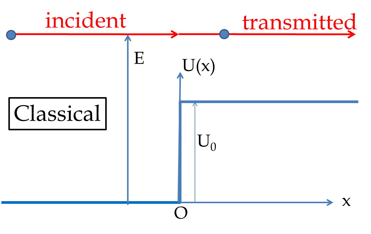
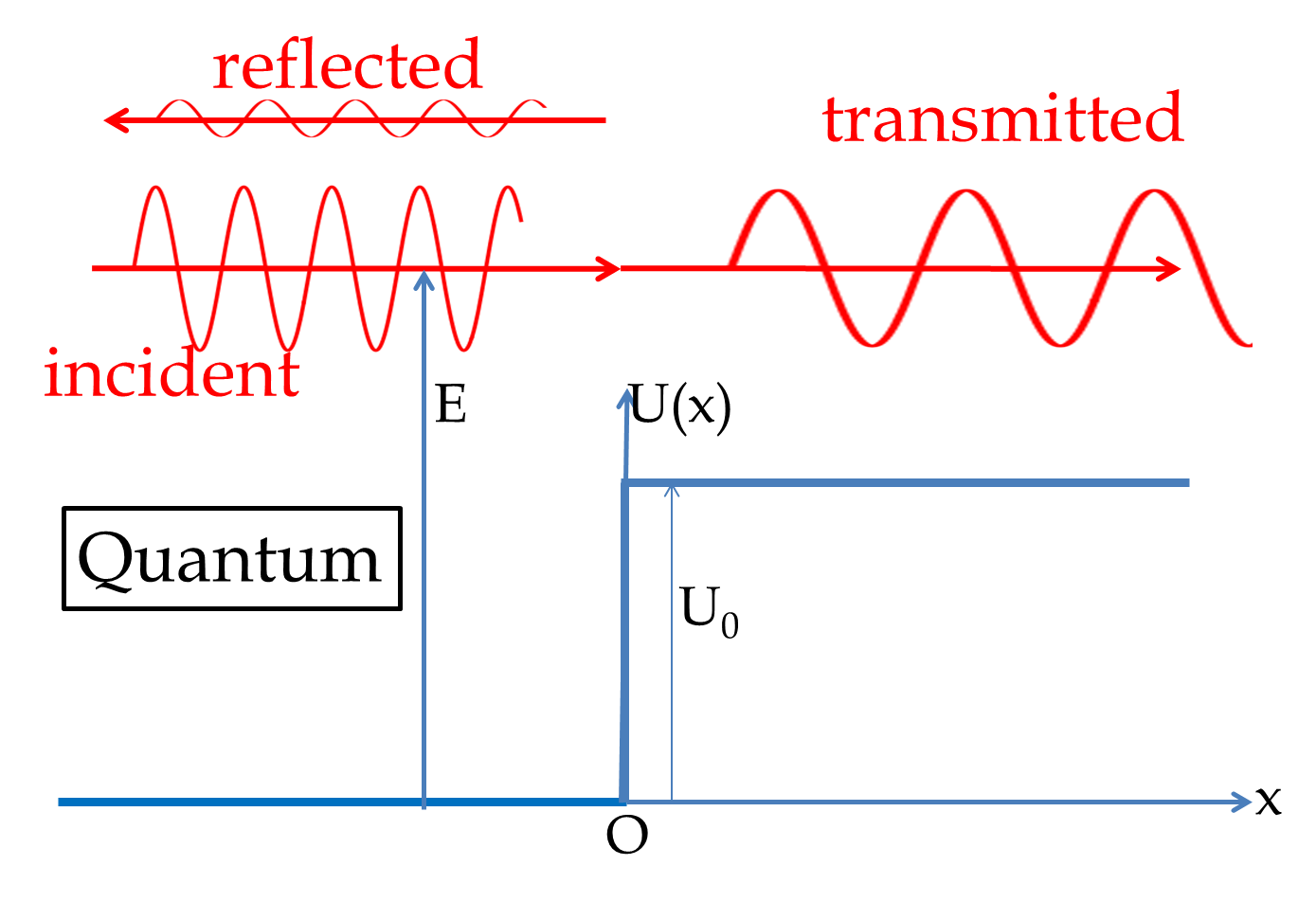
If energy \(E\) of the particle is more than the potential energy of the barrier \(U_0\text{,}\) then in the classical world of everyday life such as plane flying over a mountain, the particle will just continue onward. But in quantum mechanics, the wave function in the \(x \lt 0\) region will be a superposition of a wave moving towards the positive \(x\)-axis, \(\psi_\text{in}\text{,}\) and another wave moving towards the negative \(x\)-axis, \(\psi_\text{re}\text{.}\)
\begin{equation*}
\psi_I = \psi_\text{in} + \psi_\text{re}.
\end{equation*}
In the region \(x>0\) we have one wave - the transimtted wave moving towards the positive \(x\)-axis, \(\psi_\text{tr}\text{.}\)
\begin{equation*}
\psi_{II} = \psi_\text{tr}.
\end{equation*}
To write the solutions it is better to introduce the following constants.
\begin{equation*}
k = \dfrac{\sqrt{2mE}}{\hbar},\quad k' = \dfrac{\sqrt{2m(E-U_0)}}{\hbar}, \quad \omega = \dfrac{E}{\hbar}.
\end{equation*}
In terms of these constants the incoming, reflected and transmitted waves are:
\begin{equation*}
\psi_\text{in} = A e^{ikx-i\omega t},\quad \psi_\text{re} = B e^{-ikx -i\omega t}, \quad \psi_\text{tr} = C e^{ikx-i\omega t},
\end{equation*}
where \(A\text{,}\) \(B\text{,}\) and \(C\) are the amplitudes of the incoming wave, the reflected wave, and the transmitted wave. The wave function in the two regions are:
\begin{align*}
\amp \psi_I(x,t) = A e^{ikx-i\omega t} + B e^{-ikx -i\omega t}.\\
\amp \psi_{II}(x,t) = C e^{ikx-i\omega t}.
\end{align*}
The wave functions in the two regions join at \(x=0\) such that they have same amplitudes and same slopes with respect to \(x\) at \(x=0\text{.}\) These are called boundary conditions on the wave function.
\begin{align}
\amp \psi_I(0,t) = \psi_{II}(0,t) \longrightarrow A + B = C.\tag{51.29}\\
\amp \left.\dfrac{d\psi_I}{dx}\right|_{x=0} = \left.\dfrac{d\psi_{II}}{dx}\right|_{x=0} \longrightarrow A - B = \dfrac{k'}{k}C. \tag{51.30}
\end{align}
\begin{equation*}
\dfrac{B}{A} = \dfrac{k-k'}{k+k'},\quad\quad \dfrac{C}{A} = \dfrac{2k}{k+k'}.
\end{equation*}
The probability current of incoming wave tells us the flux of the incoming wave. Suppose there is a source of particles at \(x=-\infty\text{,}\) then the number of particles arriving at \(x=0\) per unit time will be proportional to \(j_\text{in}\text{.}\) In that experiment, the particle leaving \(x=0\) towards \(x=-\infty\) will be \(j_\text{re}\) and towards \(x=\infty\) will be \(j_\text{tr}\text{.}\) Therefore, the flux of reflected and transmitted waves should add up to the flux of the incoming wave. Let us verify this by computing the probability currents for the three waves.
\begin{equation*}
j_\text{in} = \dfrac{\hbar A^2 k}{m},\quad j_\text{re} = -\dfrac{\hbar B^2 k}{m}, \quad j_\text{tr} = \dfrac{\hbar C^2 k'}{m}.
\end{equation*}
Therefore,
\begin{equation*}
\left|\dfrac{j_\text{tr}}{j_\text{in}} \right| = \dfrac{k'C^2}{kA^2},\quad \left|\dfrac{j_\text{re}}{j_\text{in}} \right| = \dfrac{B^2}{A^2}.
\end{equation*}
This gives the desired conservation of probabilities arrivig at \(x=0\) and leaving \(x=0\) as expected.
\begin{equation*}
\left|\dfrac{j_\text{tr}}{j_\text{in}} \right| + \left|\dfrac{j_\text{re}}{j_\text{in}}\right| = \dfrac{k'C^2}{kA^2} + \dfrac{B^2}{A^2} = 1.
\end{equation*}
