   
Logo image

Physics Bootcamp

Section 44.8 Image in Two-lens Systems

In many instruments two or more lenses, sometimes in combnation with mirrors and prisms, are used one after another to form the final image, which can be a real image on a screen or a detector or a virtual image that you would view.
In this section, we will address the issue of finding the location, orientation, and magnification of the final image in the case of two-lens systems. We can do this either by ray tracing method or algebraic method.
Procedure: In both ray tracing and algebraic methods, we work one lens at a time. first we locate the image, say \(I_1\) of the object from the first lens, completely ignoring the presence of second lens. Then, we take this image to be the object for the second lens and locate the final image \(I_2\text{.}\) Clearly, this iterative process can continue for any number of optical elements, whether you have lenses or mirrors.

Subsection 44.8.1 Ray Tracing in a Two-Lens System

As an illustrative example consider a convex lens (lens \(\text{L}_1\)) followed by a concave lens (lens \(\text{L}_2\)) as shown in Figure 44.64. Here, \(\text{F}_{ij}\) refers to the focal point \(i=(1 \text{ or } 2\text{,}\) for first and second focal points) of the \(j^\text{th}\) lens. That is, \(\text{F}_{12}\) is the first focal point of the lens number 2.
I have placed the object \(\text{OP}\) within a focal length of lens \(\text{L}_1\) so that we will get a virtual image, which is guaranteed to form to the left of \(\text{L}_1\) and \(\text{L}_2\text{.}\) This is easier case than the case in which image from \(\text{L}_1\) forms on the right of lens \(\text{L}_2\text{.}\) In the present example, I have drawn rays \(11'\) and \(22'\) to locate the image of point \(\text{P}\) at \(\text{Q}_1\) by lens \(\text{L}_1\text{.}\)
Then, I have used \(\text{Q}_1\) as object with lens \(\text{L}_1\) removed. That is, I have pretended that lens \(\text{L}_1\) isn’t even there, and drawn rays \(33'\) and \(44'\) for refraction by \(\text{L}_2\) only. The backward extensions of \(3'\) and \(4'\) gives us the image of \(\text{Q}_1\) at \(\text{Q}_2\text{.}\) This is the final image of \(\text{P}\text{.}\) The image is virtual.
Figure 44.64. Ray tracing in a two-lens optical system.

Subsection 44.8.2 Algebraic Method for Two-Lens System

We work one lens at a time, making sure that we follow the sign convention given Section 44.7. Let us work out the example in Figure 44.64 with the following numerical values where \(d\) is the separation between the lenses. I have drawn the figure with the following values.
\begin{align*} \amp f_1 = 8.0\text{ cm},\\ \amp f_2 = -4.0\text{ cm},\\ \amp d = 10.0\text{ cm},\\ \amp p = 5.0\text{ cm}. \end{align*}
From \(f_1\) and \(p\text{,}\) we get \(q_1\text{.}\)
\begin{equation*} \frac{1}{q_1} = \frac{1}{8} - \frac{1}{5} = -\frac{3}{40}. \end{equation*}
Therefore, \(q_1 = -40/3\text{ cm} = -13.3\text{ cm}\text{.}\) Now, this image is to serve as object for \(\text{L}_2\text{.}\) The “object” is to the left of \(\text{L}_2\text{,}\) therefore, object distance will be positive. We need to include the distance between the two lenses to get the distance of this “object” to \(\text{L}_2\text{.}\) Therefore, for \(\text{L}_2\text{,}\) we have
\begin{align*} \amp p_2 = d + |q_1| = 10 + \frac{40}{3} = \frac{70}{3}\text{ cm}.\\ \amp f_2 = -4.0\text{ cm}. \end{align*}
Using these we get \(q_2\) by
\begin{equation*} \frac{1}{q_2} = -\frac{1}{4} - \frac{3}{70} = -\frac{82}{470}. \end{equation*}
Therefore, \(q_2 = -5.7\text{ cm}\text{.}\)
We can work out the magnification step by step also. In lens \(\text{L}_1\text{,}\) the magnification occured by the following factor.
\begin{equation*} m_1 = -\frac{q_1}{p} = -\frac{-40}{3\times 5} = +\frac{8}{3}. \end{equation*}
In lens \(\text{L}_2\text{,}\) the magnification occured by
\begin{equation*} m_2 = -\frac{q_2}{p_2} = -\frac{-470}{82} \times \frac{3}{70} = +0.25. \end{equation*}
Therefore, the net magnification will be a product of these two.
\begin{equation*} m = m_1\times m_2 = \frac{8}{3} \times 0.25 = 0.67. \end{equation*}
Thus, final image will be upright and about two-thirds of the size of the object. In Figure 44.64 the image looke like half the size. That’s because it is really difficult to draw rays accurately. While ray tracing, you would need to be very careful with the sketch if you want an accurate result.

Exercises 44.8.3 Exercises

1. Image by Two Convex Lenses.

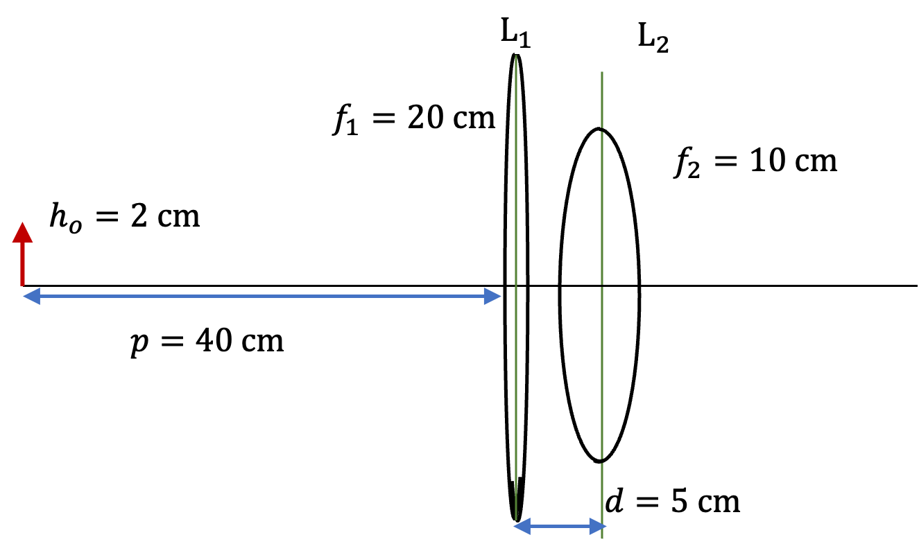
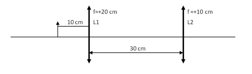
Two convex lenses of focal lengths \(20\text{ cm}\) and \(10\text{ cm}\) are placed \(30\text{ cm}\) apart as shown in Figure 44.65. An object of height \(2\text{ cm}\) is placed \(10\text{ cm}\) in front of the lens of the focal length \(20\text{ cm}\text{.}\) Find the location, orientation and magnification factor of the final image.
Figure 44.65. Figure for Exercise 44.8.3.1.
Hint.
Work one lens at a time.
Answer.
\(12.5\ \text{cm}\) back of lens L2, inverted, half the size, \(h_i = 1.0 \text{ cm}\text{.}\)
Solution.
We will work one lens at a time. First we find the image from lens L1 and use this image as object for lens L2. We have the following for lens L1.
\begin{equation*} p = +10\ \text{cm},\ \ f = + 20\ \text{cm}. \end{equation*}
Therefore, the image distance \(q_1\) will be
\begin{equation*} \frac{1}{q} = \frac{1}{20\ \text{cm}} - \frac{1}{10\ \text{cm}} = -\frac{1}{20\ \text{cm}} \ \ \Longrightarrow q_1 = -20\text{ cm}. \end{equation*}
Therefore, the image by lens L1 will be virtual and at \(20\text{ cm}\) to the left of the L1.
Now, we take the image from L1 and treat it like an object for lens L2. To get the object distance to L2, we need to include the distance between the lenses also.
\begin{equation*} p_2 = |q_1| + d = 20\text{ cm} + 30\text{ cm} = 50\text{ cm}. \end{equation*}
with \(f_2= + 10\text{ cm}\text{,}\) we get
\begin{equation*} \ \frac{1}{q_2} = \frac{1}{10\ \text{cm}} - \frac{1}{50\ \text{cm}}\ \ \Longrightarrow\ \ q_2 = 12.5\ \text{cm}. \end{equation*}
Therefore, the location of the final image is \(12.5\ \text{cm}\) back of lens L2.
To find the net magnification, we find magnification in each lens and then multily them.
\begin{align*} \amp m_1 = -\frac{q_1}{p} = -\frac{-20\ \text{cm}}{10\ \text{cm}} = + 2. \\ \amp m_2 = -\frac{q_2}{p_2} = -\frac{12.5\ \text{cm}}{50\ \text{cm}} = - 1/4. \\ \amp m = m_1\times m_2 = -\frac{1}{2}. \end{align*}
Hence, the final image is inverted and is half the size of the original object. That, is the size of the image is \(1\text{ cm}\text{.}\)

2. Image by Two Convex Lenses with Intermediate Image Behind Second Lens.

Two convex lenses of focal lengths \(20\text{ cm}\) and \(10\text{ cm}\) are placed \(5\text{ cm}\) apart as shown in Figure 44.66. An object of height \(2\text{ cm}\) is placed \(40\text{ cm}\) in front of the lens of the focal length \(20\text{ cm}\text{.}\) Find the location, orientation and magnification factor of the final image.
Figure 44.66. Figure for Exercise 44.8.3.2.
Hint.
Work one lens at a time. The intermediate image will be to the right of L2. that will mean \(p_2\) will be negative.
Answer.
\(\frac{70}{9}\ \text{cm}\) back of lens L2, inverted, \(\frac{2}{9}\) of the size of object, \(h_i = \frac{4}{9} \text{ cm}\text{.}\)
Solution.
We will work one lens at a time. First we find the image from lens \(\text{L}_1\) and use this image as object for lens \(\text{L}_2\text{.}\) We have the following for lens \(\text{L}_1\text{.}\)
\begin{equation*} p = +40\ \text{cm},\ \ f = + 20\ \text{cm}. \end{equation*}
Therefore, the image distance \(q_1\) will be
\begin{equation*} \frac{1}{q} = \frac{1}{20\ \text{cm}} - \frac{1}{40\ \text{cm}} = \frac{1}{40\ \text{cm}} \ \ \Longrightarrow q_1 = 40\text{ cm}. \end{equation*}
Therefore, the image by lens \(\text{L}_1\) will be real and at \(40\text{ cm}\) to the right of the \(\text{L}_1\text{.}\)
Now, we take the image from \(\text{L}_1\) and treat it like an object for lens \(\text{L}_2\text{.}\) To get the object distance to \(\text{L}_2\text{,}\) we need to include the distance between the lenses also. From the geometry we see that the image from \(\text{L}_1\) will fall to the right of \(\text{L}_2\text{.}\) Therefore, the object distance here will be negative.
\begin{equation*} p_2 = -(|q_1| - d) = -35\text{ cm}. \end{equation*}
with \(f_2= + 10\text{ cm}\text{,}\) we get
\begin{equation*} \ \frac{1}{q_2} = \frac{1}{10\ \text{cm}} - \frac{1}{-35\ \text{cm}}\ \ \Longrightarrow\ \ q_2 = \frac{70}{9}\ \text{cm}. \end{equation*}
Therefore, the location of the final image is \(\frac{70}{9}\ \text{cm}\) back of lens \(\text{L}_2\text{.}\) That is the final image will be a real image.
To find the net magnification, we find magnification in each lens and then multily them.
\begin{align*} \amp m_1 = -\frac{q_1}{p} = -\frac{40\ \text{cm}}{40\ \text{cm}} = -1. \\ \amp m_2 = -\frac{q_2}{p_2} = -\frac{70}{9}\times\frac{1}{-35}=\frac{2}{9}. \\ \amp m = m_1\times m_2 = -1\times \frac{2}{9} = - \frac{2}{9}. \end{align*}
Hence, the final image is inverted and is \(\frac{2}{9}\) the size of the original object. That, is the size of the image is \(\frac{4}{9}\text{ cm}\text{.}\)

3. Virtual Image Through a Two-Convex Lens System.

Two convex lenses of focal lengths \(25\, \text{cm}\) and \(10\, \text{cm}\) are placed \(59\, \text{cm}\) apart. An object of height \(2\, \text{cm}\) is placed \(50\, \text{cm}\) in front of the lens of focal length \(25\, \text{cm}\text{.}\) Find the location, orientation and magnification factor of the final image.
Answer.
\(q_{\textrm{final}} = 90\, \text{cm}\) to the left of \(\text{L}_2\text{,}\) \(m = -10\text{.}\)
Solution.
We will work one lens at a time and with the convention that the object is placed to the left of 1 and lens 2 is to right of lens 1. Let us denote the properties associated with the two lenses by the subscripts 1 and 2 respectively.
\begin{equation*} \textrm{Given: } f_1 = 25\:\textrm{cm},\ \ p_1 = 50\:\textrm{cm},\ \ \textrm{we find }\ q_1 = + 50\:\textrm{cm}. \end{equation*}
Since \(q_1 \gt 0\) the image is \(50\, \text{cm}\) to the right of lens 1. The magnification of this intermediate image is
\begin{equation*} m_1 = \dfrac{h_{i1}}{h_{o1}} = -\dfrac{q_1}{p_1} = -\dfrac{50}{50} = -1. \end{equation*}
Since \(m_1 \lt 0\) the image is inverted. Now, this intermediate image will be the object for the lens 2. This gives
\begin{equation*} p_2 = 59-50= 9\:\textrm{cm},\ \ f_2 = +10\:\textrm{cm}. \end{equation*}
Therefore
\begin{equation*} \dfrac{1}{9} + \dfrac{1}{q_2} = \dfrac{1}{10},\ \ \Longrightarrow\ \ q_2 = -90\:\textrm{cm}. \end{equation*}
Since \(q_2 \lt 0\) this image is \(90\,\text{cm}\) to the left of lens 2. The magnification in lens 2 is
\begin{equation*} m_2 = \dfrac{h_{i2}}{h_{o2}} = -\dfrac{q_2}{p_2} = -\dfrac{-90}{9} = +10. \end{equation*}
Therefore, the net magnificaiton is
\begin{equation*} m = m_1\: m_2 = (-1)(+10) = -10. \end{equation*}
The final image will be \(10\) times larger and inverted. The final image will be \(90\,\text{cm}\) to the left of lens 2 which means that the final image will be \(31\, \text{cm}\) to the left of lens 1. This is a virtual image. That means you would see it if you look from behind lens \(\text{L}_2\text{.}\)

4. Image formed by a Two-Convex Lens System.

Two convex lenses of focal length \(35\,\text{cm}\) and \(5\,\text{cm}\) are placed \(41\,\text{cm}\) apart. An object of height \(2\,\text{cm}\)is placed \(5000\,\text{cm}\) in front of the lens of focal length \(35\,\text{cm}\text{.}\) Find the location, orientation and magnification factor of the image.
Answer.
\(q = 38.3\, \text{cm}\) behind \(\text{L}_2\text{,}\) \(m = +0.05\text{.}\)

5. A Diverging and Converging Two-Lens System.

An object of height \(3\, \text{cm}\) is placed at \(25\, \text{cm}\) in front of a diverging lens of focal length \(20\, \text{cm}\text{.}\) Behind the diverging lens there is a converging lens of focal length \(20\, \text{cm}\text{.}\) The distance between the lenses is \(5\, \text{cm}\text{.}\) Find the location, orientation and size of the final image.
Answer.
\(83\,\text{cm}\) to the right of \(\text{L}_2\text{,}\) \(m = -2.3\text{,}\) \(h_i= 6.9\, \text{cm}\text{.}\)
Solution.
In this problem lens 1 is a diverging lens. Therefore we have
\begin{equation*} \textrm{Given: } f_1 = -20\:\textrm{cm},\ \ p_1 = 25\:\textrm{cm},\ \ \textrm{we find }\ q_1 = -\dfrac{100}{9}\:\textrm{cm}. \end{equation*}
Since \(q_1 \lt 0\) the image is \(\dfrac{100}{9}\:\textrm{cm}\) to the left of lens 1. The magnification of this intermediate image is
\begin{equation*} m_1 = \dfrac{h_{i1}}{h_{o1}} = -\dfrac{q_1}{p_1} = -\dfrac{-100/9}{25} = +\dfrac{4}{9}. \end{equation*}
Since \(m_1 \gt 0\) the image has the same vertical orientation as the object. Now, this intermediate image will be the object for the lens 2. This gives
\begin{equation*} p_2 = 5\:\textrm{cm}-(-\dfrac{100}{9}\:\textrm{cm})= \dfrac{145}{9}\:\textrm{cm},\ \ f_2 = +20\:\textrm{cm}. \end{equation*}
Therefore, \(q_2 = 82.9\:\textrm{cm}\text{.}\) Since \(q_2 \gt 0\) this image is \(82.9\, \text{cm}\) to the right of lens 2. The magnification in lens 2 is
\begin{equation*} m_2 = \dfrac{h_{i2}}{h_{o2}} = -\dfrac{q_2}{p_2} = -\dfrac{82.9}{145/9} = -5.14. \end{equation*}
This says that the image of the intermediate image is magnified and inverted with respect to the intermediate image. Therefore, the net magnification is
\begin{equation*} m = m_1\: m_2 = \left( \dfrac{4}{9} \right)(-5.14) = -2.3. \end{equation*}
The final image will be \(2.3\) times larger than the original object and inverted. The height of the final image will be \(6.9\, \text{cm}\text{.}\)

6. Ray Tracing Through Two Convex Lenses.

Copy Figure 44.67 and draw rays accurately to find the image of the object OP.
Figure 44.67.
Solution.
It turns out that the final image and the intermediate image in the given figure are too close to each other since the intermediate image forms almost on top of the second lens. In the following figure, Figure 44.68, I have moved the second lens a little bit to the right compared the figure above. This gives a better view of the intermediate image.
The basic idea is to work with one lens at a time. Use the image by the first lens as an object of the second lens and get new special rays to work with for the lens 2. If you had more than two lenses, you would repeat this process.
Figure 44.68.

7. Ray Tracing Through a Convex Concave Combo.

Copy the figure Figure 44.69 and draw rays to find the image.
Figure 44.69.
Solution.
The ray tracing is shown in Figure 44.70.
Figure 44.70.

8. Ray Tracing Through a Convex Concave Combo.

Copy the figure Figure 44.71 and draw rays to find the image.
Figure 44.71.

9. Ray Tracing Through a Two Convex Combo.

Copy the figure Figure 44.72 and draw rays to find the image.
Figure 44.72.