   
Logo image

Physics Bootcamp

Section 39.3 Inductance in Circuits

Every circuit with a changing current has an induced back EMF due to the self-inductance of the circuit. The back EMF opposes the change in current and therefore, slows down rise and drop in current levels. In this section we will study simple circuits with only inductance and resistance. In another chapter we will study AC circuits that have sinusoidally varying currents and include capacitance as well.
Rising Current in an RL-Circuit
To study the effect of self-inductance, consider a circuit in which a source of constant EMF, such as a battery, is connected to a solenoid through a switch as shown in Figure 39.18.
Let there be no current in the circuit before the switch S is closed at say, \(t=0\text{.}\) We will show here that current in the circuit does not come full strength right away - it takes some time before current builds up in the circuit. At what rate does the current rise?
Figure 39.18.
When the switch is closed, the current in the circuit will be increasing for some time. The changing current will cause a change in the self magnetic flux through the circuit, which will induce a back EMF opposing the rising current. Eventually, the current will reach a maximum steady value. From that point on in time, the induced EMF will be zero since the self magnetic flux will be unchanging.
Using Calculus, we will work out Eq. (39.12) below that tells us current at instant \(t\text{.}\)
\begin{equation} I(t) = I_{\text{max}}\left(1-e^{-\frac{R}{\mathcal{L}}t} \right),\tag{39.9} \end{equation}
where \(I_{\text{max}} = \mathcal{E}_0/R,\) \(R\) is the net resistance in the circuit, and \(L\) is self-inductance of the circuit. The plot of current verus time in Figure 39.19 shows that the current rises exponentially with a characteristic time, given by the ratio of self-inductance \(\mathcal{L}\) and the resistance \(R\text{.}\)
Figure 39.19. Time dependence of current after switch is closed in circuit given in Figure 39.24.
In time \(\mathcal{L}/R\) the current rises to approximately 63\%, or more precisely, \((e-1)/e\) of the maximum. The characteristic time given by quantity \(\mathcal{L}/R\) is called the inductive time constant \(\tau\) of the circuit, and can be used to determine how quickly the circuit reaches the steady state.
\begin{equation*} \tau = \mathcal{L}/R. \end{equation*}
For instance, in a circuit with \(1\, \text{k}\Omega\) resistance, and \(1\text{ H}\) self-inductance, the time-constant \(\tau\) will be \(1\text{ msec}\text{.}\) For \(R\) in Ohms and \(\mathcal{L}\) in Henry, the time constant \(\tau\) will be in seconds.
\begin{equation*} [\tau] = \frac{[\mathcal{L}]}{[R]} = \frac{\text{H}}{\Omega}=\frac{\Omega.\text{s}}{\Omega} = \text{s}. \end{equation*}
Turning off Current in an RL-Circuit
Opening a switch in an inductive circuit can be dangerous and must be done with care, since the current in such a circuit cannot be turned off from some value \(I_{\text{max}}\) to zero instantaneously. To safely open a circuit with a large inductance, you will need to give the circuit some time for the current to decay.
This is usually done by leaving a resistor in series with the inductor when switching off the power supply as shown in Figure 39.20. The current is diverted to a circuit without the power source.
Figure 39.20.
Faraday flux rule for the new loop of current with no source in Figure 39.20 is
\begin{equation*} R I(t) = -\mathcal{L} \frac{dI}{dt}, \end{equation*}
with initial condition \(I(0) = I_0\text{.}\) The solution of this equation is readily obtained.
\begin{equation} I(t) = I_0 e^{-\frac{R}{\mathcal{L}}t}.\tag{39.10} \end{equation}
The solution tells us that the current will decease in the circuit with the same time constant \(\tau = \mathcal{L}/R\) once the power source is disconnected as we found for the rise in the current when the power is turned on.

Example 39.21. Time Constant of an \(RL\) Circuit.

Self-inductace of an electric motor is \(10\,\text{H}\text{.}\) Th motor is connected in a circuit of net resistance \(200.0\,\Omega\text{.}\) What is the time constant of this circuit?
Solution.
From the formula \(\tau = \mathcal{L}/R\) we get
\begin{equation*} \tau = \frac{10\,\text{H}}{200.0\,\Omega} = \frac{1}{20}\,\text{sec}. \end{equation*}

Subsection 39.3.1 Energy Dissipation in RL-circuit

Energy in a circuit is dissipated in the resitors of the circuit. You have studied before that when a current \(I\) is flowing through a resitor of resistance \(R\text{,}\) the rate of energy dissipation is
\begin{equation*} P = VI, \end{equation*}
where \(V\) is the voltage across the resistor. If current is a function of time, we call this instantaeous power and denote it by
\begin{equation*} P(t) = I(t)V(t). \end{equation*}
Now, in an LR-circuit, when we open the circuit safely by letting the current flow through a circuit with only a resitor \(R\) and an inductor \(\mathcal{L}\) in series, we will get
\begin{equation*} P(t) = I(t)V(t) = R I_0^2 e^{-2\frac{R}{\mathcal{L}}t}, \end{equation*}
where I have used \(V=IR\) and the formula for \(I(t)\) from Eq. (39.10). Now, if we want to know how much energy will be dissipated in \(t=t_1\) to \(t=t_2\text{,}\) we will need to integrate \(P(t)\text{.}\) This will give
\begin{equation*} \Delta U = \frac{1}{2}\mathcal{L}I_0^2\left( e^{-2\frac{R}{\mathcal{L}}t_1} - e^{-2\frac{R}{\mathcal{L}}t_2} \right). \end{equation*}
If \(t_2\) is taken to be \(\infty\text{,}\) this would give a measure of energy present in the circuit at instant \(t_1\text{.}\)
\begin{equation*} U(t_1) = \frac{1}{2}\mathcal{L}I_0^2\,e^{-2\frac{R}{\mathcal{L}}t_1}. \end{equation*}
At \(t_1=0\text{,}\) we can interpret that the circuit with steady current \(I_0\) has energy
\begin{equation*} U(t=0) = \frac{1}{2}\mathcal{L}I_0^2. \end{equation*}

Example 39.22. Power Dissipation in an \(RL\) Circuit.

A motor of self-inductance \(\mathcal{L} = 10\,\text{H}\) shown as coil in Figure 39.23 is connected in a circuit with a resistor of resistance \(R_1=200.0\,\Omega\text{,}\) a dissipative resitor \(R_2=1000.0\,\Omega\) and a battery of voltage \(V=9.0\,\text{V}\) using a switch. In the ON position, switch connects \(R_1\) and battery to the motor and in the OFF position, only \(R_2\) is connected to the motor.
Figure 39.23.
(a) The switch is in the ON position for a long time. (i) What is the time constant of this circuit? (ii) How much current flows at the peak? (iii) How much energy is stored in this circuit at the peak current? (b) The switch is now thrown into the OFF position. (i) What is the time constant of this circuit? (ii) How long will it take for half of the energy to be dissipated in this circuit?
Solution 1. a
(i) The time constant is easily worked out to be \(\mathcal{L}/R_1\text{.}\)
\begin{equation*} \tau_1 = \frac{\mathcal{L}}{R_1} = \frac{10}{200} = \frac{1}{20}\,\text{sec}. \end{equation*}
(ii) The peak current is when all voltage of the battery falls across the resistor \(R_1\text{.}\)
\begin{equation*} I_\text{max} = \frac{V}{R_1} = \frac{9}{200}\,\text{A}. \end{equation*}
Solution 2. b
(i) Now, the active circuit has only \(\mathcal{L}\) and \(R_2\text{.}\) Hence, the time constant is
\begin{equation*} \tau_2 = \frac{\mathcal{L}}{R_2} = \frac{10}{1000} = \frac{1}{100}\,\text{sec}. \end{equation*}
(ii) The time constant for power dissipation is twice the time constant.
\begin{equation*} U(t) = U_0\, e^{-t/(\tau_2/2)}. \end{equation*}
We need \(t\) when \(U(t)=\frac{1}{2}\,U_0\text{.}\) Therefore,
\begin{equation*} \frac{1}{2} = e^{-t/(\tau_2/2)}. \end{equation*}
Taking natural log of both sides we get
\begin{equation*} t = \frac{\tau_2}{2}\,\ln\,2 = 3.47\,\text{msec} \end{equation*}

Subsection 39.3.2 (Calculus) Current After Closing Switch in an Inductive Circuit

We are interested in understanding how the current develops in Figure 39.18 from zero at the zero of time to the steady current value. Since we are interested in the time-changing aspect of the circuit, we will use Faraday’s flux rule to write the loop equation as opposed to the Kirchhoff’s loop equation, which is valid only in steady circuits. For Faraday’s flux rule we will need to evaluate a line integral of the electric field around the circuit.
\(\)
This is aided by redrawing the physical circuit given in Figure 39.18 as a conceptual circuit and displaying the net resistance in the circuit by a resistor of resistance \(R\) and the self-inductance \(\mathcal{L}\) by an element in the circuit as shown in Figure 39.24.
Figure 39.24.
You might think of \(\mathcal{L}\) as a solenoid in the circuit whose self-inductance dominates the self-inductance of the circuit. Such elements in the circuit are called inductors - they are assumed to have zero resistance and \(\int\vec E\cdot d\vec l = 0\) across them. They only give rise to the EMF through the flux change through their loops. Performing the line integral of electric field \(\vec E\) in the direction of the current shown in Figure 39.24 gives us
\begin{equation*} \oint\vec E\cdot d\vec l = -\mathcal{E}_0 + I(t) R\ \ \text{(Going in the direction of the current)}. \end{equation*}
By Faraday’s law, this must be equal to the negative of the rate of change of magnetic flux through the circuit, which is given by the following from the definition of self-inductance.
\begin{equation*} \frac{d\Phi_{\text{self}}}{dt} = \mathcal{L} \frac{dI}{dt}. \end{equation*}
Therefore, you get the following equation for the current in the loop.
\begin{equation} -\mathcal{E}_0 + I(t) R= -\mathcal{L}\frac{dI}{dt}. \tag{39.11} \end{equation}
The solution of Eq. (39.11) with \(I(0) = 0\) will tell us how the current develops in the circuit. We have solved this type of differential equation in the context of charging of a capacitor. The answer can be obtained readily by analogy.
\begin{equation} I(t) = I_{\text{max}}\left(1-e^{-\frac{R}{\mathcal{L}}t} \right),\tag{39.12} \end{equation}
where
\begin{equation*} I_{\text{max}} = \frac{\mathcal{E}_0}{R}. \end{equation*}

Subsection 39.3.3 Inductors in Series and Parallel

\(\,\)
Series: When inductors are in series (Figure 39.25) the EMF induced across them are induced by the same current.
Therefore, the induced EMF in each will be
\begin{equation*} \mathcal{E}_1 = L_1 \dfrac{dI}{dt},\ \ \mathcal{E}_2 = L_2 \dfrac{dI}{dt}. \end{equation*}
Figure 39.25.
The net EMF across the two inductors in series will be the sum of the two EMFs.
\begin{equation*} \mathcal{E} = \mathcal{E}_1 + \mathcal{E}_2 = \left( L_1 + L_2 \right)\: \dfrac{dI}{dt} = L_{\text{series}}\:\dfrac{dI}{dt}. \end{equation*}
Thus,
\begin{equation} L_{\text{series}} = L_1 + L_2.\tag{39.13} \end{equation}
Parallel: In a parallel connections (Figure 39.26) the EMF across the two inductors will be same but will be generated by two different currents.
\begin{align*} \amp I = I_1 + I_2,\\ \amp \mathcal{E} = L_1 \dfrac{dI_1}{dt},\ \ \mathcal{E} = L_2 \dfrac{dI_2}{dt}. \end{align*}
Figure 39.26.
We can deduce the following relation between the EMF induced \(\mathcal{E}\) and net current \(I\text{.}\)
\begin{equation*} \mathcal{E} = \left( \dfrac{L_1L_2}{L_1 + L_2} \right)\: I. \end{equation*}
Therefore, we can define the equivalent inductance for parallel circuit as
\begin{equation*} L_{\text{parallel}} = \dfrac{L_1 L_2}{L_1 + L_2}. \end{equation*}
We can write this in more familiar form.
\begin{equation} \dfrac{1}{L_{\text{parallel}}} = \dfrac{1}{L_1} + \dfrac{1}{L_2}.\tag{39.14} \end{equation}

Example 39.27. Variation of Current in an RL-Circuit.

A \(12\text{-V}\) battery is connected to a \(10\text{-mH}\) inductor and a \(50\text{-}\Omega\) resistor at \(t = 0\text{.}\) Find the following: (a) the inductive time constant, (b) the current at \(t = 0\text{,}\) (c) the current as \(t \rightarrow \infty\text{,}\) (d) the time for the current to reach quarter of the maximum.
Answer.
(a) \(0.2\; \text{msec}\text{,}\) (b) \(0\text{,}\) (c) \(0.24\: \text{A}\text{,}\) (d) \(58\: \mu\text{s} \text{.}\)
Solution 1. a
The time constant of an RL-circuit is
\begin{equation*} \tau = \dfrac{\mathcal{L}}{R} = \dfrac{10 \text{ mH}}{50\, \Omega} = 0.2\text{\, msec}. \end{equation*}
Solution 2. b
Since a current through an inductor cannot change abruptly since that would imply infinite back EMF. That means current through an inductor is a continuous function of time. Therefore, \(I = 0\) for \(t\lt 0\) would imply that \(I=0\) at \(t=0\text{.}\)
Solution 3. c
Current reaches a steady state as \(t \rightarrow \infty\text{,}\) and there will be no induced EMF in the circuit. Setting \(dI/dt = 0\) in Faraday’s flux rule yields,
\begin{align*} I_{\text{max}} \amp = \mathcal{E}_0/R \\ \amp = 12\: \text{V}/50\: \Omega = 0.24\: \text{A}. \end{align*}
Solution 4. d
To find the time to reach one-fourth of the maximum current we set \(I(t) = \dfrac{1}{4}\,I_{\text{max}}\) and solve the resulting equation for \(t\text{.}\)
\begin{equation*} \frac{I_{\text{max}}}{4} = I_{\text{max}}\left( 1 - e^{-t/\tau}\right). \end{equation*}
Simplifying this equation gives
\begin{equation*} e^{-t/\tau} = 3/4. \end{equation*}
Taking the natural logarithm of both sides yields
\begin{equation*} t = -\tau\ln{(0.75)} = 58\: \mu\text{s}. \end{equation*}

Example 39.28. Time for Current to Decay and Energy Dissipated in an RL-Circuit.

A \(100\text{-V}\) source is connected to a \(1.0\, \text{k}\Omega\) resistor and a \(30\, \text{H}\) coil and the current is allowed to reach maximum. A switch is then thrown that disconnects the voltage source at \(t = 0\text{,}\) but leaves the resistor and the inductor connected in another loop.
Figure 39.29.
(a) Determine the time it will take for the current in the circuit to drop to \(10\%\) of its value at \(t = 0\text{.}\) (b) How much energy is dissipated in that time?
Answer.
(a) \(69\ \text{ms}\text{,}\) (b) \(4.95\ \text{mJ}\text{.}\)
Solution 1. (a)
Let us first find the time constant for the circuit since it will be needed in the problem.
\begin{equation*} \tau = \dfrac{L}{R} = \dfrac{30\:\text{H}}{1000\:\Omega} = 0.03\:\text{sec}. \end{equation*}
The time for the current to drop to 10\% of max will obey the following equation.
\begin{equation*} 0.1\:I_{\text{max}} = I_{\text{max}}\:e^{-t/\tau}. \end{equation*}
This gives
\begin{equation*} t = -0.03\:\ln(0.1) = 69\:\text{ms}. \end{equation*}
Solution 2. (b)
We need \(I_{\text{max}}\) at \(t=0\text{,}\) therefore we seek
\begin{equation*} I_{\text{max}}= \dfrac{V}{R} = \dfrac{100\:\text{V}}{1000\:\Omega} = 0.1\:\text{A}. \end{equation*}
The energy dissipated is the difference of energy at \(t=0\) and at \(t=0.069\: \text{sec}\text{.}\)
\begin{align*} \Delta U \amp = \dfrac{1}{2}\: L\:\left[ I_{\text{max}}^2 - (0.1\: I_{\text{max}})^2\right]\\ \amp = \dfrac{1}{2}\times 0.99\times 0.1^2 = 4.95\:\text{mJ}. \end{align*}

Exercises 39.3.4 Exercises

1. Computing Currents in an RL Circuit.

The switch in the circuit given in Figure 39.30 is closed at \(t = 0\text{.}\) Determine current through each resistor as \(t \rightarrow \infty\text{.}\)
Figure 39.30. Exercise 39.3.4.1
Hint.
When steady state is reached, you can ignore the inductance.
Answer.
\(I = 0.257\:\text{A}\text{,}\) \(I_1 = 0.171\:\text{A}\text{,}\) \(I_2 = 0.086\:\text{A}\)
Solution.
With time the circuit approaches steady state. In the steady state, the current does not change, which means that there would be no self-inductance as \(t\rightarrow \infty\text{.}\)
If there is no self-inductance, we can ignore the presence of inductor in the circuit. The circuit simplifies to the resistors only as shown in Figure 39.31.
Figure 39.31.
The equivalent circuit when steady state has reached can be readily solved for currents from techniques you have learned before. The current through the battery is simple the voltage of the battery divided by the equivalent resistance of the circuit.
The equivalent resistance is
\begin{equation*} R_{eq} = 20\,\Omega + \frac{40\,\Omega\times 80\,\Omega}{40\,\Omega+ 80\,\Omega} = 46.7\,\Omega. \end{equation*}
Therefore, current through the battery is
\begin{equation*} I = \frac{12\:\text{V}}{46.7\:\Omega} = 0.257\:\text{A}. \end{equation*}
Since a parallel circuit is a current divider, currents in the two branches are
\begin{align*} \amp I_1 =\left( \frac{80\,\Omega}{40\,\Omega+ 80\,\Omega}\right) 0.257\:\text{A} = 0.171\:\text{A}\\ \amp I_2 =\left( \frac{40\,\Omega}{40\,\Omega+ 80\,\Omega}\right) 0.257\:\text{A} = 0.086\:\text{A} \end{align*}

2. Numerical RL-Circuit.

A \(200\text{-}\Omega\) resistor is connected to a \(2\text{-mH}\) inductor and a \(10\text{-V}\) source in series. The voltage source is turned on at \(t=0\text{,}\) and the current starts to build.
(a) Determine the value of steady current.
(b) What is the voltage drop across the inductor when steady current flows through it?
(c) What is the voltage drop across the resistor at steady state?
(d) Determine the time it will take to build to \(50\%\) of the steady current in the circuit.
(e) Determine the time it will take to build \((1-1/e)\times100\%\) of the steady current.
(f) Determine the time it will take to build to \(90\%\) of the steady current.
Hint.
USe solution of series RL-circuit.
Answer.
(a) \(5.0\times 10^{-2}\, \text{A}\text{,}\) (b) \(0\text{,}\) (c) \(10\,\text{V}\text{,}\) (d) \(6.93\:\mu\text{s}\text{,}\) (e) \(10\:\mu\text{s} \text{,}\) (f) \(23\:\mu\text{s}\text{.}\)
Solution 1. a
As \(t\) becomes large we reach a steady current in the circuit given by voltage of the source and the net resistance.
\begin{equation*} I_{\text{max}} = \dfrac{V}{R} = 5.0\times 10^{-2}\:\text{A}. \end{equation*}
Solution 2. b
When current is steady, its derivative with time is zero. Hence, no voltage will drop across the inductor, assuming the inductor has only negligible resistance.
\begin{equation*} V_L = 0. \end{equation*}
Solution 3. c
Whe steady current is flowing, the circuit is like a DC circuit with resitor only. Hence, all voltage of the source must drop across the resistor.
\begin{equation*} V_R = 10\text{ V}. \end{equation*}
Solution 4. d
The time constant of an \(RL\) circuit is \(\tau = \mathcal{L}/R = 10^5\text{ s}\text{.}\) Therefore, current in the \(RL\) circuit rises according to the following
\begin{align*} I(t) \amp = I_{\text{max}}\left(1 - e^{-t/\tau} \right)\\ \amp = 0.05\:\text{A}\:\left(1 - e^{-10^5 t} \right). \end{align*}
Therefore the time to get to \(50\%\) of the max will be given by \(t\) in the following equation.
\begin{equation*} \dfrac{I}{I_{\text{max}}} = 0.5 = 1 - e^{-10^5 t}. \end{equation*}
You can solve this for \(t\) by rearranging and taking natural log of both side.
\begin{equation*} \ln(e^{-10^5 t}) = \ln(1-0.5). \end{equation*}
This gives
\begin{equation*} t = \frac{\ln(2)}{10^{5}} = \frac{0.693}{10^5} = 6.93\times 10^{-6}\,\text{sec}. \end{equation*}
Hence, \(t=6.93\:\mu\text{s}\text{.}\)
Solution 5. e
\begin{equation*} I_{\text{max}}\left(1 - e^{-1} \right) = I_{\text{max}}\left(1 - e^{-10^5t} \right) \text{ gives } \end{equation*}
This gives \(t= 10\,\mu\text{s}.\)
Solution 6. f
Now, time \(t\) will satisfy the following condition.
\begin{equation*} 0.9\:I_{\text{max}}\left(1 - e^{-1} \right) = I_{\text{max}}\left(1 - e^{-10^5 t} \right) \end{equation*}
This gives
\begin{equation*} t= 23\, \mu\text{s}. \end{equation*}

3. (Calculus) Numerical Study of Current Rise and Magnetic Energy Storage in a Coil.

A coil of resistance \(0.2\,\Omega\) and inductance \(0.4\, \text{mH}\) is connected across a battery of voltage \(12\,\text{V}\) and internal resistance \(0.01\,\Omega\) and a switch S. The coil has radius \(5\, \text{cm}\) and length \(30\, \text{cm}\text{.}\) The switch is closed at \(t =0\text{.}\)
(a) Find the time it will take the current to reach \(99\%\) of its final value. (b) Find the amount of energy transferred to the coils as heat during that time? (c) How much energy is stored in the coils as magnetic field at \(t=4\,\text{msec}\text{?}\) (d) (Calculus) At what rate is the current increasing at \(t = 4\, \text{msec}\text{?}\)
Hint.
(a) Use series \(RL\) circuit equations. (b) Resistance of coils is important here. (c) Use magnetic energy formula. (d) Need \(dI/dt\) - you can use solution \(I(t)\) and take derivative.
Answer.
(a) \(9.2 \times 10^{-4}\ \text{sec}\text{,}\) (b) 0.6 J, (c) 0.54 J, (d) \(4.1 \times 10^3\ \text{A/s}\text{.}\)
Solution 1. (a)
Recall the solution of a series LR-circuit is
\begin{equation*} I(t) = I_{\text{max}}\:\left(1 - e^t/\tau \right), \ \ \ \ \ \ (1) \end{equation*}
with
\begin{equation*} I_{\text{max}} = \dfrac{V}{R},\ \ \tau = \dfrac{L}{R}. \end{equation*}
Setting \(I = 0.99\; I_{\text{max}}\) in Eq. (1) gives
\begin{equation*} 0.99 = 1 - e^{-t/\tau}. \end{equation*}
Solving this equation for \(t\) we find
\begin{align*} t \amp = \tau \ln(100) \\ \amp = \dfrac{0.4\times 10^{-3}\:\text{H}}{0.2\:\Omega}\:\ln(100) = 9.2\times 10^{-4}\:\text{s}. \end{align*}
For use in the second part of this exercise let us denote this time by letter \(T\text{.}\)
\begin{equation*} T \equiv 9.2\times 10^{-4}\:\text{s}. \end{equation*}
Solution 2. (b)
The energy spent in this time can be obtained by integrating the instantaneous power.
\begin{align*} W \amp = \int P dt = \int I^2 R dt\\ \amp = \dfrac{V^2}{R}\:\int_0^T\: \left( 1 - 2 e^{-Rt/L} + e^{-2Rt/L} \right)\: dt. \end{align*}
The integrals are easy to do and the result comes out to be
\begin{equation*} W = \dfrac{V^2}{R}\left[ T + \dfrac{2L}{R}\left( e^{-RT/L} -1 \right) -\dfrac{L}{2R} \left( e^{-2RT/L} -1 \right) \right]. \end{equation*}
Putting in the numerical values we find \(W = 0.6\:\text{J}\text{.}\)
Solution 3. (c)
Here
\begin{equation*} I(\text{at }4\:\text{ms}) = \dfrac{12}{0.2}\left(1 - e^{-500\times 0.004}\right) = 52\:\text{A}. \end{equation*}
Therefore,
\begin{align*} U \amp = \dfrac{1}{2}LI^2\\ \amp = \dfrac{1}{2}\times 0.4\times 10^{-3} \times 52^2 = 0.54\:\text{J}. \end{align*}
Solution 4. (d)
A direct calculation on (1) yields
\begin{equation*} \frac{dI}{dt} =\frac{V}{R} \frac{R}{L}\: e^{-Rt/L}. \end{equation*}
Putting in the numerical values gives \(4.1\times 10^3\: \text{A/s}\text{.}\)

4. (Calculus) Voltage Drop Across a Coil with Changing Current.

A large coil of inductance \(200\text{ H}\) is connected to a varying current source such that current passing through the coil is given by \(I = 120\text{ A }\cos(400 t)\text{.}\) Find the voltage across the inductor.
Hint.
Voltage reading is equal to the EMF induced.
Answer.
\(9.6\times 10^6\sin(400\:t) \text{ V}\text{.}\)
Solution.
The voltage across an inductor is equal to the EMF induced in the coil when current is varying with time.
\begin{align*} V \amp = L\dfrac{dI}{dt}\\ \amp = -200\times 120\times 400\times \sin(400\:t) = 9.6\times 10^6\:\sin(400\:t)\:\text{V}. \end{align*}

5. (Calculus) Different Time Constants in Different Branches of an RL-Circuit.

The switch in the given circuit is closed at \(t=0\text{.}\) Find currents in the circuit as functions of time and describe how different currents in the circuit develop with time.
Figure 39.32.
Hint.
Set up KCL and Farady equations in the circuit. Solve the resuting differential equation.
Answer.
\(I_1 = 2\,\text{ A}\text{,}\) \(I_2 = 2\, \text{A}\, \left( 1 - e^{-t/4}\right)\text{,}\) \(I = 2\,\text{A} + 2\,\text{A}\, \left( 1 - e^{-t/4}\right)\text{.}\)
Solution.
We will apply Kirchhoff’s Current Law (KCL) to the nodes and Faraday’s flux rule to the loops since we have time-changing current and there is an inductor in the circuit. If a loop does not contain an inductor then we will ignore the induced EMF due to the circuit since the induced EMF would be negligible for those circuits.
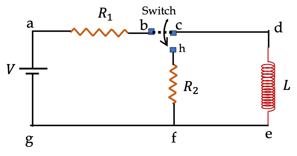
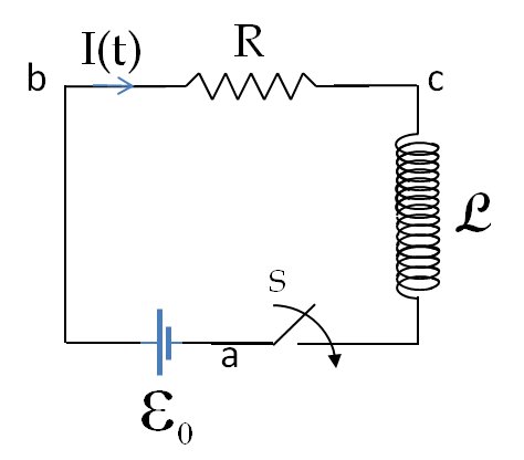
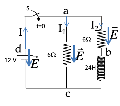
We start with labelling nodes of the circuit, which are a, b, and c. We have added one more label, d, to help describe the loop on the left side. We then assign currents in the branches beginning with the current in the source, which we take from negative to the positive.
We will need the directions of the electric field in various elements of the circuit. As shown in the figure, electric field is in the direction of the current in the resistors and opposite to the direction of current in the battery. We assume that the solenoid is ideal in the sense that it has a zero resistance, or, the resistance of the solenoid is lumped with the other resistance in its branch.
Now, we can write relations among currents as follows.
\begin{align} \amp \text{Currents at node a: }\ \ I = I_1 + I_2 \tag{39.15}\\ \amp \text{Loop a-c-d-a: }\ \ +6I_1 - 12 = 0 \tag{39.16}\\ \amp \text{Loop a-b-c-a: }\ \ +6I_2 - 6I_1= -24 \frac{dI_2}{dt} \tag{39.17} \end{align}
Note the last equation includes the induced EMF due to the changing of current \(I_2\) through the inductor. These equations have to be solved together to find the three currents. Fortunately, current \(I_1\) is independent of time as given by Eq. (39.16).
\begin{equation*} I_1 = 2\ \text{A}. \end{equation*}
This says that current \(I_1\) comes on instantaneously when the switch is turned on. That is, the time constant for this current is zero and there is no delay on reaching the maximum current in this branch since we have ignored minute self-inductance in the loop without the coils.
To find \(I_2\text{,}\) we replace \(I_1\) in Eq. (39.17) and rearrange the result to
\begin{equation*} \frac{dI_2}{dt} + \frac{1}{4} I_2 = \frac{1}{2}. \end{equation*}
Note that this equation would have been obtained also from the loop a-b-c-d-a. The solution of this equation is
\begin{equation*} I_2 = 2 A \left( 1 - e^{-t/4}\right). \end{equation*}
The current \(I_2\) in the branch on the right side in the circuit does not attain the maximum value of 
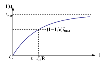
\(2\text{ A}\) instantaneously, but it takes time due to the inductor in this branch. Initially, current is zero in this branch at \(t=0\text{.}\) When the source attempts to force current through this branch, the back EMF opposes the rise in the current. The time constant for this current is \(4\,\text{sec}\text{.}\) Finally, the current through the battery is obtained by using Eq. (39.15).
\begin{equation*} I = 2\text{ A} + 2\text{ A } \left( 1 - e^{-t/4}\right) \end{equation*}
The current through the battery rises instantaneously to \(2\,\text{ A}\text{,}\) but takes time to get to the final value of \(4\, \text{A}\) due to the inductor in the circuit.