Resonance in Driven Circuits

Section 40.4 Resonance in Driven Circuits

An important point about the driven circuit in the steady state is that its dynamical quantities such as voltage across the capacitor, current in the circuit, and power delivered to the resistor depend upon the driving frequency, which we can control in the experiment. When you vary the driving frequency, amplitudes as well as phases of oscillations of these quantities can be varied by wide margins. In each case, there is a special frequency at which the amplitude is the largest. This phenomenon is called resonance and the frequency at which the amplitude is the largest is called the resonance frequency of that quantity.

Subsection 40.4.1 Resonance of Voltage Across Capacitor

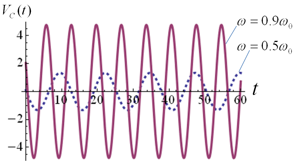
An important point about the driven circuit in the steady state is that the voltage across the capacitor depends on the driving frequency \(\omega\) in relation to the natural frequency \(\omega_0\text{.}\) The situation here is analogous to the situation of a swing in children’s playground - the amplitude of swing depends on the frequency with which one pushes on it. By keeping \(R\text{,}\) \(L\) and \(C\) fixed, i.e. keeping the circuit same, we can vary the frequency of the driving EMF, and look at the voltage across the capacitor after the steady state has reached. For each driving frequency \(\omega\text{,}\) we find that the peak voltage across the capacitor is different as shown in Figure 40.32.

Figure 40.32. Voltage across the capacitor versus time. Note the value of the peak voltage depends on the driving frequency \(\omega\text{.}\) The two curves are for two values of driving frequency: the solid line corresponds to \(\omega = 0.9\omega_0\) and the dashed line for \(\omega = 0.5\omega_0\text{.}\) The other parameters are same for the two plots: \(R = 0.1\ \Omega\text{,}\) \(L\) = 1 H, \(C\) = 1 F, \(V_0\) = 1 V.

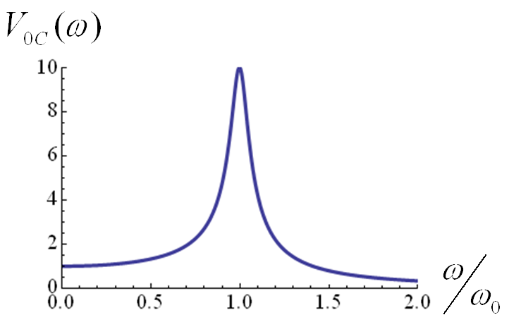
An interesting question then arises: how does the peak voltage \(V_{0C}\) vary with the driving frequency \(\omega\text{.}\) We have already found the answer to this question. The analytic expression for \(V_{0C}\) is given in Eq. (40.41). In Figure 40.33 I have plotted \(V_{0C}\) versus \(\omega\) to show you what the dependence looks like graphically.

Figure 40.33. Resonance curve of the capacitor voltage. The amplitude of oscillations of the voltage across the capacitor plates is plotted versus frequency of the EMF source. We find the amplitude of is maximum for a particular value of the frequency of the source EMF. The following values were kept fixed in the plot: \(R = 0.1\ \Omega\text{,}\) \(L\) = 1 H, \(C\) = 1 F, \(V_0\) = 1 V.

We find that there is a driving frequency at which the peak voltage across the capacitor has the largest value. We say that the peak voltage of capacitor resonates at this frequency, and call the frequency \(\omega_C\) the resonance frequency of the peak voltage across the capacitor. We will find below that the current in the circuit also depends in a similar manner on the driving frequency and exhibits a resonance phenomena, but the resonance frequency \(\omega_I\) for the current is different than the resonance frequency \(\omega_C\) for the voltage across the capacitor.

By using calculus we can predict where the resonance frequency will occur by setting the derivative of \(V_{0C}(\omega)\) with \(\omega\) to zero and solving this equation for \(\omega\text{.}\) We find the the independent variable \(\omega\) appears only in the denominator. Therefore, instead of taking the derivative of \(V_{0C}\) we can get the same result by actually taking the derivative of the quantity inside the radical in the denominator.

\begin{equation*} \frac{dV_{0C}}{d\omega} = 0 \ \ \ \Longrightarrow\ \ \ \frac{d}{d\omega}\left[ \omega^2R^2C^2+\left( \omega^2 LC-1\right)^2\right] = 0 \end{equation*}

This equation yields the following for the resonance frequency \(\omega_C\text{.}\)

\begin{equation*} \omega_C = \sqrt{\frac{1}{LC}-\frac{R^2}{2L^2} }, \end{equation*}

which can also be written as

\begin{equation*} \omega_C = \omega_0\: \sqrt{1-\frac{1}{2}\omega_0^2\tau_C^2}, \end{equation*}

where \(\tau_C = RC\) and \(\omega_0 = 1/\sqrt{LC}\text{.}\) The resonance frequency of \(V_C\) can also be expressed in terms of the Q-factor of the oscillator by noting that

\begin{equation*} Q \approx \frac{\omega_0}{2\beta} = \frac{1}{R}\: \sqrt{\frac{L}{C}}=\frac{1}{\omega_0\tau_C}. \end{equation*}

Therefore, the resonance frequency \(\omega_C\) of \(V_C\) is given as

\begin{equation*} \omega_C =\omega_0\: \sqrt{1-\frac{1}{2}\omega_0^2\tau_C^2}= \omega_0\sqrt{1-\frac{1}{2Q^2}}. \end{equation*}

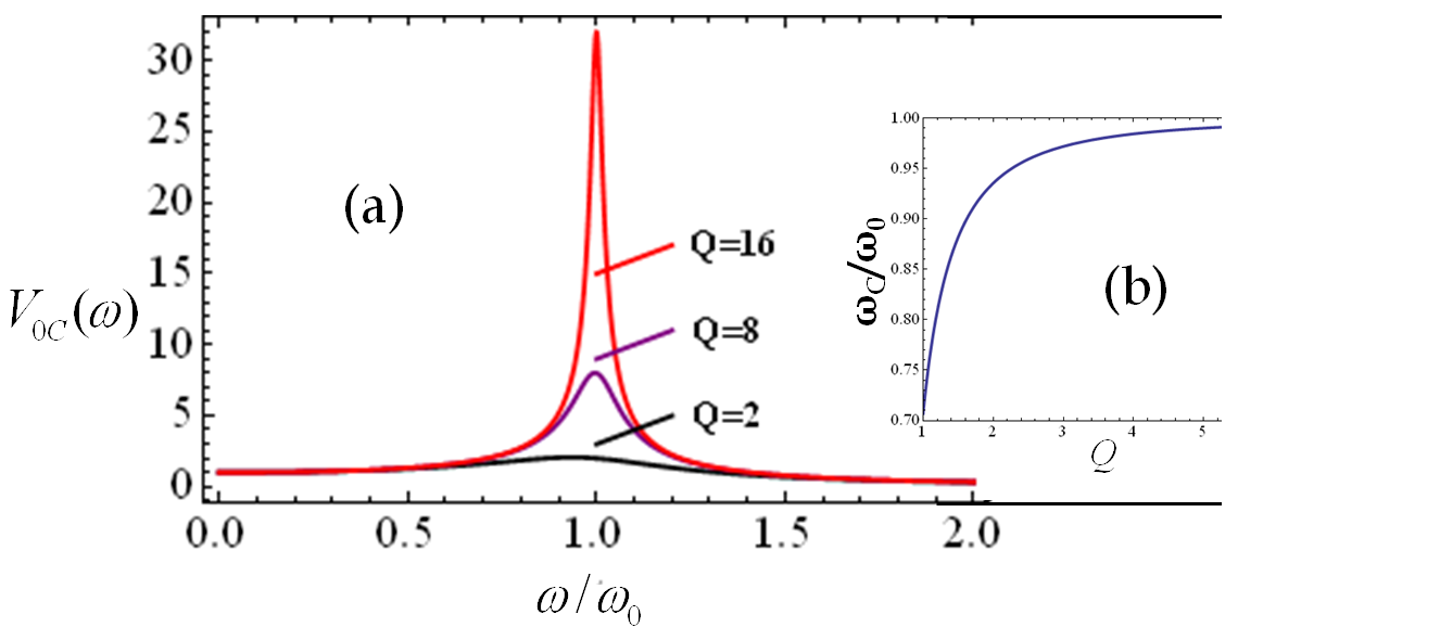
The sharpness of the resonance curve depends on how good the oscillator is in maintaining its oscillations as given by the Q-factor of the oscillator. Figure 40.34 shows plots of the resonance curves for various values of the Q-factor. As the Q-factor increases, the oscillator becomes a better oscillator, the plot of the peak voltage versus the driving frequency becomes sharper, and the resonance frequency of \(V_C\) moves closer to \(\omega_0\) as shown in the figure.

Figure 40.34. (a) Plot of the amplitude of the voltage across the capacitor as a function of the driving frequency for \(Q=2,\) \(8\text{,}\) and \(16\text{.}\) (b) The resonance frequency \(\omega_C\text{,}\) here the ratio \(\omega_C/\omega_0\) as a function of Q shows that resonance frequency tends to the natural frequency \(\omega_0\) as Quality factor \(Q\) of the oscillator rises.

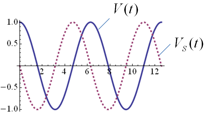
Significance of the Phase Angle The driving EMF V(t) and the steady state capacitor voltage \(V_S\) have a difference of phase angle \(\phi\text{.}\) What does the angle \(\phi\) mean? One way to look at \(\phi\) is that it tells us about the lag or lead of the phase of the oscillation of the voltage across the capacitor with respect to the oscillation of the driving EMF. To get a better feel of what the difference does, we plot the driving EMF (\(V\)) and the steady state capacitor voltage (\(V_S\)) in Figure 40.35 for \(\phi =+\pi/2\) rad for amplitude and angular frequency, \(\omega = 1\ \textrm{rad/sec}\text{.}\) The plot shows that the maxima of the \(V_S(t)\) in this example occur before that of \(V(t)\text{.}\) We say that \(V_S(t)\) leads \(V(t)\text{.}\) The lead here is a quarter of the cycle since \(\phi = \pi/2\) and the full cycle corresponds to an angle \(2\pi\) rad.

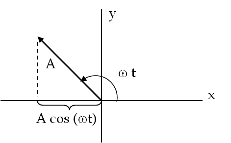
Figure 40.35. Illustration of EMF \(V=\cos(t)\) and \(V_s=\cos(t+\phi)\) for \(\phi= +\pi /2\) rad.

An easier way to observe the phase difference is through the use of a polar plot, called the phasor diagram. Note that a sinusoidal function can be represented by components of a vector, the \(x\)-component for cosine and the \(y\)-component for the sine. To compare two sinusoidal functions in their vector representations, first you must convert all the sines and cosines to either all sines or all cosines. In our present study we will convert them all into cosines. Then, the \(x\)-component of these vectors will contain the physical information. In Figure 40.36, the vector diagram of \(A \cos(\omega t)\) is shown by an arrow pointed in the counterclockwise direction at an angle \(\omega t\) from the positive \(x\)-axis.

Figure 40.36. The function \(A cos (\omega t)\) represented as the \(x\)-component of a vector in a phasor diagram. The fictitious vector for representing a cosine or a sine function in this way is called a phasor.

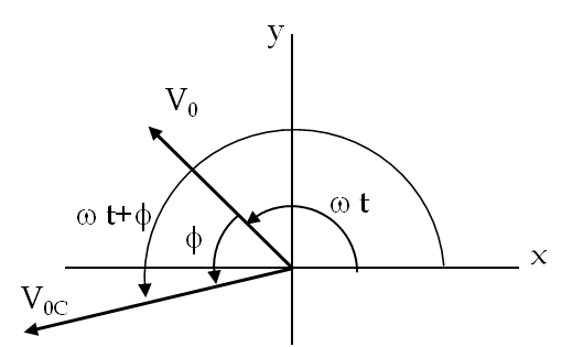
The vector rotates counterclockwise in time in keeping with the argument \(\omega t\) of cosine. The vector is called a phasor. When phasors corresponding to the driving EMF and the steady state voltage across the capacitor are plotted in the same diagram, the two phasors point in different directions, although both rotate at the same rate. If angle \(\phi \gt 0\text{,}\) then the phasor for \(V_S\) is said to be ahead of the phasor for \(V\text{,}\) while the opposite is the case when \(\phi \lt 0\text{.}\) In Figure 40.37, you can examine a situation in which phasor \(V_S\) is ahead of phasor V.

Figure 40.37. Phasor diagram of two phasors drawn on the same diagram for comparing the phases of two cosine or sine functions. Here the phasor of the driving EMF \(V\) represents the function \(V_0\cos(\omega t)\) and the phasor for \(V_S\) represents the function \(V_0\cos(\omega t + \phi)\) for a positive \(\phi\text{.}\)

Subsection 40.4.2 Dependence of Phase on the Driving Frequency

We have discussed above how the peak capacitor voltage \(V_{0C}\) in a series RLC-circuit driven by a sinusoidal EMF depends on the driving frequency. We found that there is a particular frequency when the resonance of \(V_C(t)\) takes place in the circuit. The phase difference of \(V_C(t)\) from the driving EMF \(V(t)\) also depends on the driving frequency which we rewrite here.

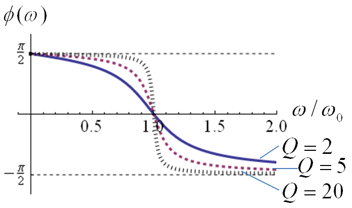
\begin{equation} \tan(\phi) = \frac{1}{\omega\tau_C} - \omega\tau_L,\tag{40.42} \end{equation}

where \(\tau_C = RC\) and \(\tau_L = L/R\text{.}\) This dependence is shown in Figure 40.38 for \(L\) = 1 H, \(C\) = 1 F, and \(R = \frac{1}{2}\Omega\text{,}\) \(\frac{1}{5}\Omega\text{,}\) and \(\frac{1}{20}\Omega\) corresponding to Q-factors, \(Q\) = 2, 5, and 20 respectively.

Figure 40.38. Phase angle changes sign at the resonance. The sharpness of transition depends on the \(Q\)-factor of the oscillator as shown in another figure.

The plot of \(\phi\) shows a transition from \(+\pi /2\) at low frequencies to \(-\phi /2\) for high frequencies as the frequency is varied across the resonance frequency. The transition is also sharper for a circuit with a higher Q-factor. The phase \(\phi\) goes through zero at the natural frequency, i.e. when \(\omega = \omega_0\) as shown in the figure.

Subsection 40.4.3 Resonance of Current

For times \(t \gg 2\tau_L\) the current in the circuit reaches a steady state, and oscillates at the same frequency as the driving frequency as we have seen above. Let us write the steady current in the circuit as

\begin{equation*} I_S(t) = I_0\:\cos\left(\omega t + \phi + \frac{\pi}{2} \right), \end{equation*}

where the amplitude \(I_0\) and phase constant \(\phi\) depend on the driving frequency \(\omega\) as already given in the last subsection.

\begin{align} \amp I_0 = \frac{V_0}{\sqrt{R^2 + \left(\omega L-1/\omega C \right)^2}}, \tag{40.43}\\ \amp \tan(\phi) = \frac{1}{\omega\tau_C} - \omega\tau_L, \tag{40.44} \end{align}

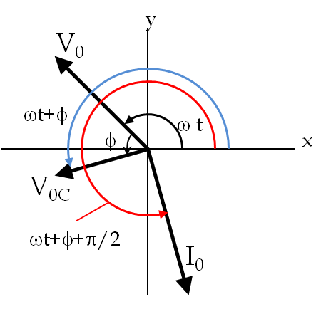
where \(\tau_C = RC\) and \(\tau_L = L/R\text{.}\) In the following we analyze the consequences of these formulas for the amplitude \(I_0\) and phase \(\omega t+ \phi + \pi/2\) of the current. The frequency dependence of \(\phi\) here is the same as that of the voltage across the capacitor \(V_C\) which has already been discussed above. In Figure 40.39, a phasor diagram has been drawn to illustrate the phases of the driving EMF, the steady capacitor voltage and the steady current.

Figure 40.39. A phasor diagram showing the driving EMF, current in the circuit and the capacitor voltage. Note that phasors rotate counterclockwise with time. The length of each phasor corresponds to the amplitude of the quantity. Since phasors in this diagram correspond to different types of physical quantities we cannot compare their lengths. However, since all three phasors rotate at the same rate \(\omega\text{,}\) the diagram provides a visual way to compare their phases or timings.

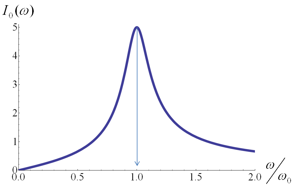
Now, we look at the amplitude \(I_0\) of the steady current as we change the angular frequency of the driving EMF. From the expression for \(I_0\) given above, you can think of \(I_0\) as a function of \(\omega\) for fixed \(V_0\text{,}\) \(R\text{,}\) \(L\) and \(C\text{.}\) For a lightly-damped oscillator, the plot of \(I_0\) versus \(\omega\) shown in Figure 40.40 clearly exhibits a maximum current when the driving EMF has a particular frequency called the resonance frequency of the current. We will use the symbol \(\omega_I\) for the resonance frequency of the current in the circuit.

Figure 40.40. Resonance of amplitude of current for \(R\) = 0.2 \(\Omega\text{,}\) \(L\)= 1 H, \(C\) = 1 F, and the peak voltage of the driving EMF set to \(V_0 = 1\) V. The peak current in the circuit is maximum when the driving frequency \(\omega\) is equal to the natural frequency \(\omega_0\) of the circuit.

From the expression for the peak current given in Eq. (40.43) we can prove analytically that the resonance frequency \(\omega_I\) is equal to \(\omega_0\text{,}\) the natural frequency. To deduce the expression for the resonance frequency of current we treat \(I_0\) as a function of \(\omega\text{,}\) set the derivative with respect to \(\omega\) to zero, and solve the equation for \(\omega\text{.}\) This gives the following for the resonance frequency of the current in the circuit.

\begin{equation*} \omega_I = \omega_0 = \frac{1}{\sqrt{LC}}. \end{equation*}

Notice that the resonance frequency of the current in the circuit is different from the resonance frequency of the capacitor voltage. Other aspects of the resonance of \(I\) are similar to the resonance of \(V_C\) and we will not discuss them.

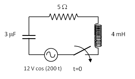
Example 40.41. Current and Voltages in a Series RLC Circuit.

Consider the circuit in Figure 40.42. (a) Find the steady current and voltages across the resistor and the capacitor in the circuit for \(t \gg 2L/R\text{.}\)

(b) Find the resonance frequency of current. (c) Compare the energy dissipated in the resistor at the frequency shown in the figure to the energy dissipated if driven at the resonance frequency.

Solution 1. a

The steady current is \(I = I_0\: \cos(\omega t+ \phi + \pi/2)\text{,}\) where the amplitude and phase constants are as follows in terms of \(R\text{,}\) \(L\) and \(C\) of the circuit and \(\omega\) of the driving source. But before you put in numbers, it often pays to simplify the formulas. Here \(1/\omega C\) dominates R and \(\omega L\text{.}\)

\begin{align*} \amp I_0 = \frac{V_0}{\sqrt{R^2 + (\omega L - 1/\omega C)^2}} \approx \omega C V_0= 7.2\ \textrm{mA}. \\ \amp \phi = \arctan\left( \frac{1}{\omega RC} - \frac{\omega L}{R}\right) = 1.6\ \textrm{rad}. \end{align*}

The voltage across the resistor and the capacitor are

\begin{align*} \amp V_R = RI = RI_0\: \cos(\omega t+ \phi + \pi/2) = (35\ \textrm{mV})\: \cos(\omega t+ \phi + \pi/2) \\ \amp V_C = \frac{I_0}{\omega C}\sin(\omega t+ \phi + \pi/2)= (12\ \textrm{V})\:\cos(\omega t+ \phi) \end{align*}

Solution 2. b

The resonance frequency of the current is equal to the natural frequency, \(\omega _I = \frac{1}{\sqrt{LC}} = 9129\) rad/sec.

Solution 3. c

In 1 sec the circuit goes through many cycles, and therefore we use the average power. The average energy dissipated per second = \(P_{\textrm{ave}}\times \Delta t\) = \(\frac{1}{2}I_0^2R \times 1 \textrm{sec}= 130 \mu\textrm{J}\text{.}\)

The energy dissipated at the resonance frequency would be obtained by using the value of \(I_0\) when \(\omega = \omega_I\text{,}\) the resonance frequency of the current in this circuit. This gives the following value.

\begin{equation*} I_{0}(\omega = \omega_I) = \frac{V_0}{R} = \frac{V_0}{5\Omega} = 2.4\ \textrm{A}. \end{equation*}

Using this current in the power dissipation formula we find that the average energy dissipated at the resonance frequency in one second = \(\frac{1}{2}(2.4\ \textrm{A})^2 \times 5\Omega\times 1\) sec = 14.4 J. This is way more than the \(130 \mu\textrm{J}\) given to the resistor when driven at \(\omega = 200\) rad/sec instead of \(\omega_I = 9129\) rad/sec. Clearly, the most effective way to put energy in a circuit is to drive the circuit at the resonance frequency of the circuit.

Exercises 40.4.4 Exercises

1. Resonance Frequency of Current n RLC-Circuits.

Find the frequency at which current in each circuit will resonate.

Solution.

(a) \(\omega_R = \dfrac{1}{\sqrt{LC}} = \dfrac{1}{\sqrt{10\times 10^{-3}\:\textrm{H}\times 4\times 10^{-6}\textrm{F}}} = 5000\:\textrm{sec}^{-1}\text{.}\) This give \(f_R = \omega_R/2\pi = 796\:\textrm{Hz}\text{.}\)

(b) \(\omega_R = \dfrac{1}{\sqrt{LC}} = \dfrac{1}{\sqrt{1\times 10^{-3}\:\textrm{H}\times 20\times 10^{-6}\textrm{F}}} = 7071\:\textrm{sec}^{-1}\text{.}\) This give \(f_R = \omega_R/2\pi = 1125\:\textrm{Hz}\text{.}\)

(c) \(\omega_R = \dfrac{1}{\sqrt{LC}} = \dfrac{1}{\sqrt{4\times 10^{-3}\:\textrm{H}\times 1.6\times 10^{-6}\textrm{F}}} = 12500\:\textrm{sec}^{-1}\text{.}\) This give \(f_R = \omega_R/2\pi = 1989\:\textrm{Hz}\text{.}\)

(d) \(\omega_R = \dfrac{1}{\sqrt{LC}} = \dfrac{1}{\sqrt{5\times 10^{-3}\:\textrm{H}\times 2\times 10^{-6}\textrm{F}}} = 10000\:\textrm{sec}^{-1}\text{.}\) This give \(f_R = \omega_R/2\pi = 1592\:\textrm{Hz}\text{.}\)

2. Current Amplitude in a Driven RLC Circuit.

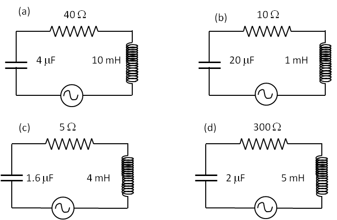
For each circuit in Exercise 40.4.4.1, find the amplitude of the current if the source has \(10\, \text{V}\) amplitude and frequency \(600\, \text{Hz}\text{.}\)

Solution.

We use the result for a series \(RLC\) circuit.

\begin{equation*} I_0 = \dfrac{V_0}{\sqrt{R^2 + (\omega L - 1/\omega C)^2}}, \end{equation*}

where \(\omega = 2 \pi f\) with \(f\) the frequency of the source EMF. Putting the numerical values from each figure we find the following values for the peak current in the four cases: (a) \(20\, \text{mA}\text{,}\) (b) \(730\, \text{mA}\text{,}\) (c) \(66\, \text{mA}\text{,}\) and (d) \(31\, \text{mA}\text{.}\)

3. Peak Current as a Function of Frequency.

For circuit (b) in Figure 40.27, plot the peak current as a function of frequency of a \(10\text{-V}\) sinusoidal source.

Solution.

We treat the peak current \(I_0\) as a function of frequency \(f\) of the driving EMF.

\begin{equation*} I_0 (f) = \dfrac{V_0}{\sqrt{R^2 + (2\pi f L - 1/2\pi f C)^2}}. \end{equation*}

Here, we have the following numerical values.

\begin{equation*} R = 10\:\Omega,\ \ L = 1\times 10^{-3}\:\textrm{H},\ \ C = 10\times 10^{-6}\:\textrm{F},\ \ V_0 = 10\:\textrm{V}. \end{equation*}

We use Mathematica® to generate the plot.

Prev Top Next